Warehouse Destratification: What a Height-Based Savings Factor Assumes About the Gradient and the Climate

Mixing Instead of Moving

Every other piece of ventilation equipment in a building moves air from somewhere to somewhere else. A destratification fan does not. It stirs air that is already in the room, and the saving it produces comes from a temperature difference that stops existing.

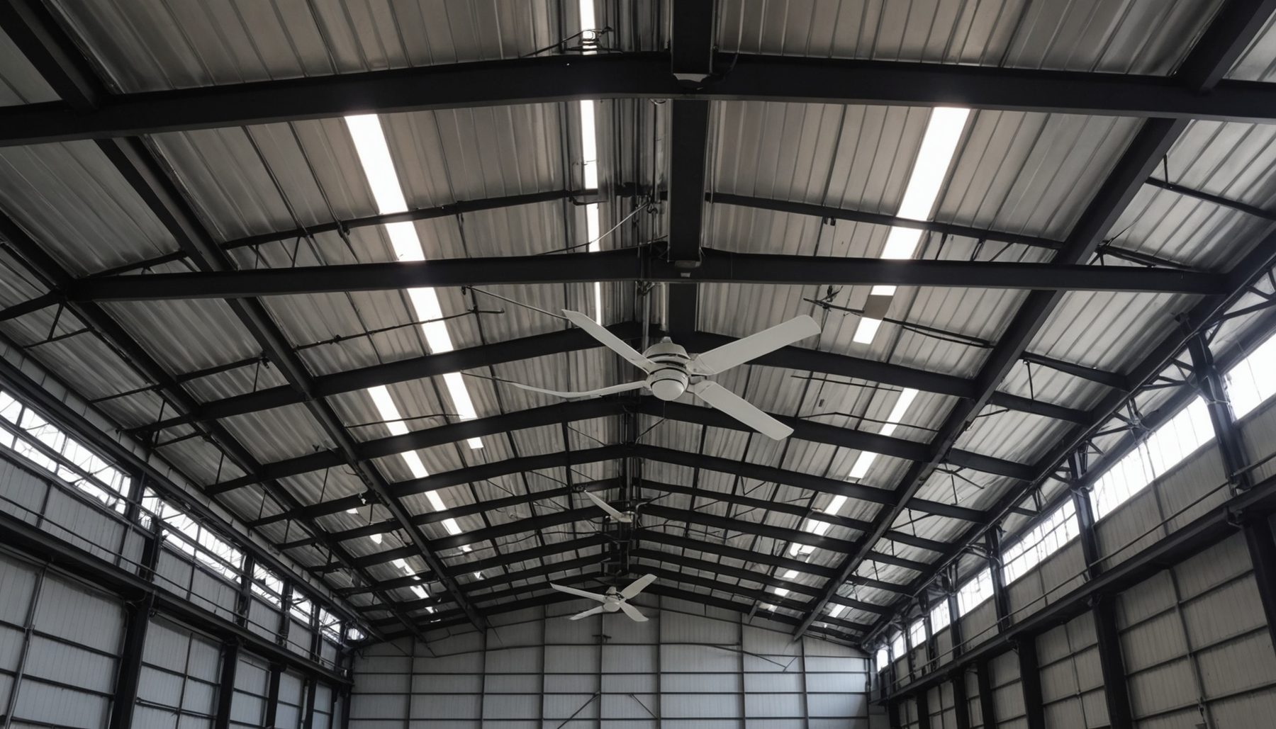
Warm air is lighter than cool air, so in a tall heated space it collects under the roof and stays there. The occupied zone at floor level sits at the temperature the thermostat is holding. The air above it sits several degrees warmer, with a gradient running between the two. The roof loses heat in proportion to the temperature of the air against it, and that air is the warmest in the building and the air nobody is using.

Stirring the space collapses the gradient. Air at floor level gets warmer because warm air has been brought down to it, which means the thermostat can be set lower to return the occupied zone to the temperature it held before. Every surface and every air path the building loses heat through then sees a smaller temperature difference, and the saving follows from that rather than from any transfer of heat into or out of the space.

The Warehouse Heating with Destratification Calculator builds a conventional heating load from the envelope, the infiltration and the ventilation, and then applies a reduction factor taken from a table indexed by eave height alone. That factor is where the whole subject sits, and it deserves closer attention than a single percentage suggests.

What follows covers where the gradient comes from and what changes it, how the composition of the load shifts as a building gets taller, what a fixed percentage implies about the temperature difference behind it, and what the page itself says about how firmly those percentages are established. The sequence of the heat loss arithmetic is set out on the calculator page and is not repeated here as the substance of the article.

Calculator Inputs: An Envelope, an Air Change Rate, a Height

The field list is a conventional heat loss calculation with one extra number in it, and the extra number carries the entire subject of this article.

Warehouse Floor Area              ft² or m²
Eave Height                       ft or m
Roof, Wall, Door and Floor        U-values with their areas
Design Indoor Temperature         °F or °C
Design Outdoor Temperature        °F or °C
Infiltration Rate                 ACH
Ventilation Airflow               CFM or m³/h, optional

Each group does one job. The areas and their U-values give the conduction losses at the design temperature difference. The air change rate turns the enclosed volume into an infiltration loss. The eave height enters twice, once through the volume that the air change rate acts on, and once as the sole index into the table of reduction factors.

The outputs follow the same division: envelope loss, infiltration loss, ventilation loss, the baseline heating load, the destratification saving in both absolute and percentage terms, the adjusted load, and the load per unit of floor area.

The reduction factor is selected from six bands. The height bands are defined in metres, an imperial height is converted before the band is chosen, and the foot figures are exact conversions of the metric cuts rather than separate boundaries:

below 3 m (9.84 ft)               D = 0.00
3 to 6 m (9.84 to 19.69 ft)       D = 0.05
6 to 9 m (19.69 to 29.53 ft)      D = 0.10
9 to 12 m (29.53 to 39.37 ft)     D = 0.15
12 to 15 m (39.37 to 49.21 ft)    D = 0.20
15 m and above (49.21 ft)         D = 0.25

The page is explicit about the standing of those values. Its formula section calls them screening assumptions used for preliminary planning rather than values prescribed by ASHRAE or any other standard, and its limitations section repeats that they are not guaranteed savings or code-prescribed figures. Realised savings, it says, depend on the vertical temperature gradient, the heating system type, fan configuration and coverage, the envelope, the climate, the controls and the operating conditions. No source for the table itself is given on the page.

What is absent from the field list is worth reading alongside that. There is no input for the vertical temperature gradient, which is the quantity mixing removes. There is no input for the heating system type, which is what the gradient depends on most strongly. There is nothing about the number, type or position of the mixing devices. And there is no check that the areas entered describe one building.

Where the Gradient Comes From

The gradient is not a property of tall buildings. It is a property of how they are heated, and the same warehouse can show a difference of a few degrees between floor and roof or of well over ten.

The mechanism is buoyancy. Warm air is less dense and rises. A heater that warms air sends it upward, and with nothing stirring the space it stays there, giving up its heat through the roof and the upper walls. What settles is a vertical temperature distribution, conventionally described as a gradient in kelvin per metre or degrees Fahrenheit per foot.

Five things move that gradient, and height is only the geometry they act over:

Heating system type. Forced air systems put heat directly into the air and produce the largest gradients. Radiant systems warm surfaces, and the air is heated secondhand from them, which gives a flatter profile.

Emitter position. Unit heaters mounted at high level reinforce stratification by releasing warm air where warm air already collects. Emitters at low level work against it.

Envelope tightness. Infiltration through dock doors admits cold air at low level, which deepens the difference between the bottom of the space and the top.

Internal gains. Lighting, process equipment and refrigeration condensers add heat at whatever level they sit at, and high-level lighting adds it where the gradient is already steepest.

Operating pattern. Night setback and morning warm-up give a different distribution from a steady state, and the largest gradients usually occur during recovery rather than at design condition.

Published values for heated high-bay spaces spread across a wide band, from a few tenths of a kelvin per metre to around one and a half, roughly 0.2 to 0.8 °F per foot. The calculator's own FAQ quotes 0.5 to 1.5 °C per metre (0.3 to 0.8 °F per foot) for a still-air warehouse. The width of that band is the point: a 12 m (39 ft) building at the bottom of it holds about 6 K (11 °F) between floor and roof, and the same building at the top holds about 18 K (32 °F).

Per ASHRAE Handbook guidance on heating high-bay spaces: vertical temperature gradients in tall heated buildings depend on the type and placement of the heating system, on envelope tightness and on internal gains, so height alone does not determine the difference between floor and roof. That quantity is not among the inputs, and the height table stands in for it.

Height Changes What the Load Is Made Of

Raising the roof of a warehouse changes the heating load in a way that is easy to state and easy to overlook. Two of the four envelope terms do not change at all, one grows in proportion to the height, and the infiltration term grows faster than any of them as a share of the total.

Working that through needs a building whose dimensions are consistent with each other, so the case below is constructed rather than scaled from the example on the calculator page:

Plan                100 × 200 ft (30.5 × 61.0 m)
Floor area          20,000 ft² (1,858 m²)
Perimeter           600 ft (183 m)
Doors               600 ft² (56 m²)
U roof / wall       0.05 / 0.07 BTU/(hr·ft²·°F)   (0.28 / 0.40 W/m²·K)
U door / floor      0.35 / 0.10 BTU/(hr·ft²·°F)   (2.0 / 0.57 W/m²·K)
Design difference   55 °F (30.6 K)
Infiltration        0.3 ACH

Four of the five terms then behave differently as the eave height H changes:

Roof    0.05 × 20,000 × 55 = 55,000 BTU/hr (16.1 kW)   fixed
Floor   0.10 × 20,000 × 55 = 110,000 BTU/hr (32.2 kW)  fixed
Doors   0.35 × 600 × 55 = 11,550 BTU/hr (3.4 kW)       fixed
Walls   0.07 × (600H − 600) × 55                       proportional to H
Inf.    0.018 × 0.3 × 20,000H × 55                     proportional to H

At three heights spanning most of the table:

                      15 ft      30 ft      45 ft
                     (4.6 m)    (9.1 m)   (13.7 m)
Roof                  55,000     55,000     55,000
Walls                 32,340     66,990    101,640
Doors                 11,550     11,550     11,550
Floor                110,000    110,000    110,000
Infiltration          89,100    178,200    267,300
Baseline load        297,990    421,740    545,490 BTU/hr
                        87.3      123.6      159.9 kW

Roof share             18.5%      13.0%      10.1%
Infiltration share     29.9%      42.3%      49.0%

Two movements are visible in those columns. Infiltration rises from under a third of the load to about half of it, because the volume it acts on grows in proportion to the height while the floor and roof areas do not. The roof falls from a little under a fifth to a tenth, because it is fixed in absolute terms while the total beneath it grows.

Now set the reduction factor beside them. It goes the other way, 0.05 at 15 ft, 0.15 at 30 ft and 0.20 at 45 ft. The factor grows over exactly the range in which the roof, the component a mixing device acts on most visibly, shrinks as a proportion of the load.

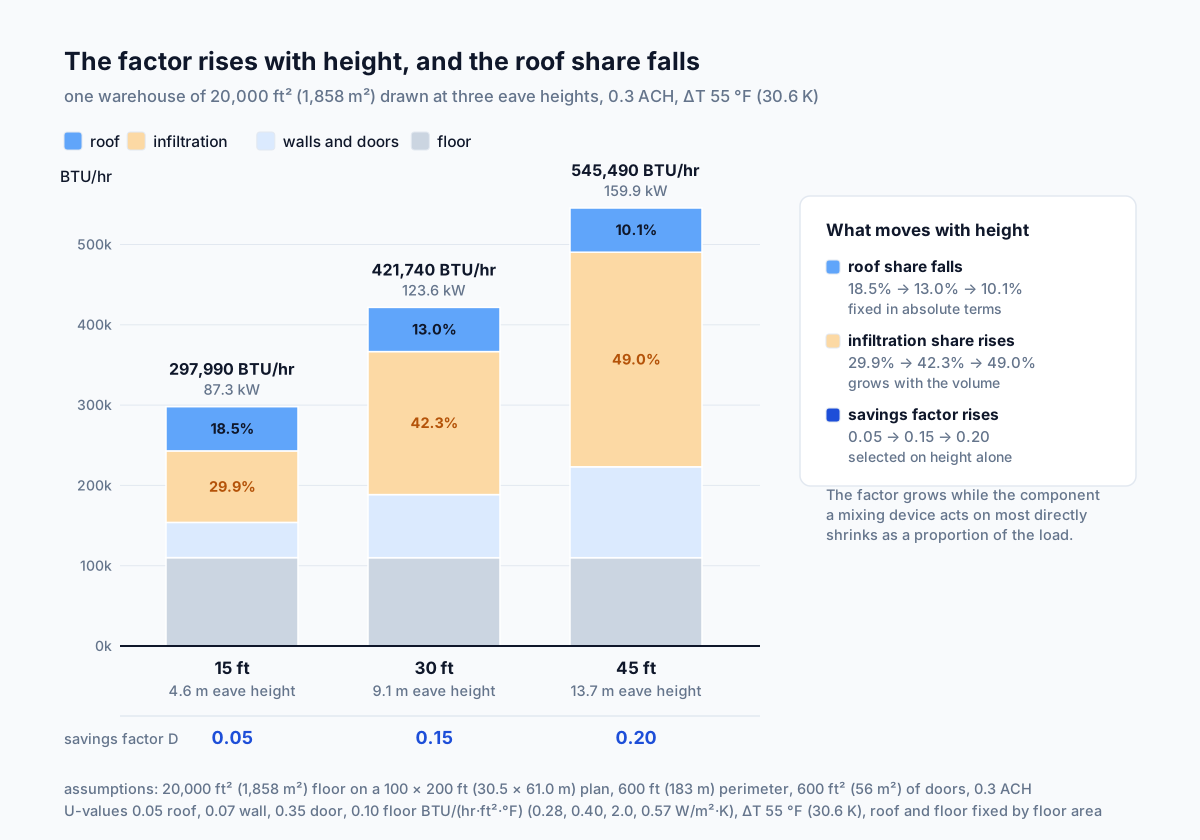
The two are reconcilable, and the way they reconcile decides how the factor should be read. If the effect of mixing is a lower thermostat setpoint, it reduces the temperature difference driving every term, and it is entirely consistent for the factor to grow while the roof share falls. If instead the effect is a cooler layer of air under the roof at an unchanged occupied-zone temperature, it belongs mostly to the roof, and a factor that grows as the roof share falls would need more explanation. Sections six and seven take that apart.

Per the structure of a heating load calculation: roof and floor losses are set by floor area and do not change with eave height, wall losses grow in proportion to it, and infiltration losses grow with the volume, so the composition of the load shifts towards infiltration as a building gets taller.

The Factor Is a Percentage, the Physics Is Degrees

The saving enters the calculation as a fraction of the load. The thing it represents is a temperature difference. Those are not the same kind of quantity, and the difference between them is where the implied design condition hides.

The factor is applied in one line:

Q_adjusted = Q_baseline × (1 − D)

where D depends on eave height alone and runs from 0.00 to 0.25 across the six bands.

Physically, what a mixing device does is level the temperature over the height of the space. The occupied zone becomes warmer, and the setpoint can then be lowered to bring it back to where it was. Lowering the setpoint is a reduction in the indoor design temperature by some number of degrees, call it δ, and every loss in the calculation is proportional to the temperature difference ΔT:

δ     equivalent setpoint reduction, K or °F     typical 1 to 6 K (2 to 11 °F)
ΔT    design temperature difference, K or °F     typical 10 to 50 K (18 to 90 °F)
D     savings factor, dimensionless               0.00 to 0.25 on this page

A reduction of δ degrees out of a difference of ΔT degrees is a saving of δ/ΔT. The fraction therefore depends on the climate, while δ does not.

Take a setpoint reduction of 4.6 K (8.3 °F), which is what the middle of the table works out at, and hold it fixed while the design condition changes:

Design difference 30.6 K (55 °F)    saving 15.0%
Design difference 11.1 K (20 °F)    saving 41.3%
Design difference 50.0 K (90 °F)    saving  9.2%

The same physical effect is worth three very different percentages. A table that returns one percentage for a given height is therefore relative to a particular design temperature difference, whether or not it says so, and if the underlying quantity really is a fixed number of degrees, the mild-climate case understates the saving and the severe-climate case overstates it.

The page states neither a design condition for its table nor a source. What it does state is that the values are screening figures and that the realised saving depends on tightness, system type and coverage. Which design difference the table was drawn up for cannot be recovered from the page, but it can be estimated from the numbers themselves.

Per the structure of the calculation: heating load is proportional to the temperature difference, so a reduction expressed as a fixed fraction and a reduction expressed as a fixed number of degrees describe the same physical effect only at one particular design temperature difference.

Working the Percentage Backwards

A percentage can be converted into the temperature difference it corresponds to. Doing that for each row of the table shows which gradient the table is consistent with, and whether that gradient is a plausible one. This is a check on applicability, not a verdict on the table.

The conversion is one multiplication:

δ = D × ΔT

δ     equivalent setpoint reduction, K
D     savings factor from the table, dimensionless
ΔT    design temperature difference, K

At a design difference of 55 °F (30.6 K), which is a common enough winter condition for a heated warehouse in a cold-temperate climate, three rows give:

15 ft (4.6 m),  D = 0.05    δ = 2.75 °F (1.53 K)
30 ft (9.1 m),  D = 0.15    δ = 8.25 °F (4.58 K)
45 ft (13.7 m), D = 0.20    δ = 11.0 °F (6.11 K)

Turning a setpoint reduction into a gradient needs one assumption, and it is a simplification: if mixing levels the space to something near its mean temperature, and the occupied zone is then returned to its original temperature, the setpoint reduction is roughly half the original floor-to-roof difference. On that basis:

Floor-to-roof difference    2δ
Implied gradient            2δ / H

4.6 m:  2 × 1.53 / 4.6  = 0.67 K/m (0.37 °F/ft)
9.1 m:  2 × 4.58 / 9.1  = 1.00 K/m (0.55 °F/ft)
13.7 m: 2 × 6.11 / 13.7 = 0.89 K/m (0.49 °F/ft)

Three rows of the table, three gradients between roughly 0.7 and 1.0 K per metre. That range sits inside the published band for heated high-bay spaces and inside the 0.5 to 1.5 °C per metre the calculator's own FAQ quotes. The table is internally coherent with a typical gradient at a design difference of the order of 30 K (54 °F).

Two things that check does not establish. It does not verify the table, because the source is unknown and the half-of-the-difference assumption simplifies a profile that is rarely linear. And it does not license replacing the table with a gradient calculation, because the published methods for estimating this effect disagree in both assumptions and results, so a home-made substitute would trade a stated screening figure for an unstated one.

What it is good for is a boundary check. If the site design difference is far from about 30 K (54 °F), or if the heating system is known to produce a flat profile, the figure the table returns deserves verification by another route before it carries a purchase decision.

Per the arithmetic of the factor and published ranges for vertical temperature gradients in heated high-bay spaces: converting each row of the table into an equivalent setpoint reduction gives gradients in the range of roughly 0.7 to 1.0 K per metre at a design temperature difference of about 30 K, which is consistent with published ranges without establishing the source of the table.

What the Factor Is Applied To

The reduction is applied to the whole baseline load, floor slab and infiltration included, and the page is careful about how that should be read. The distinction it draws matters, because the alternative reading changes the answer by tens of percent.

The model is unambiguous about the arithmetic:

Q_baseline = Q_envelope + Q_infiltration + Q_vent
Q_adjusted = Q_baseline × (1 − D)

The envelope term covers roof, walls, doors and floor slab, and the reduction is taken on the sum of all of it.

The page's own note describes the standing of that operation: the factor is applied to the total baseline load as an aggregate preliminary estimate, not as a claim that each component falls by D. Actual destratification changes the vertical temperature profile, so detailed design should evaluate roof and wall surface temperatures, infiltration conditions, heating system type and fan performance separately.

Two readings of the mechanism sit behind that caution. If mixing works through the setpoint, it lowers the indoor design temperature, which lowers ΔT, which lowers every term proportionally, infiltration included, because incoming cold air is then heated to a lower temperature. If instead mixing lowers the air temperature under the roof while the occupied zone stays where it was, the effect concentrates on the roof and upper walls and does little for the floor slab or for infiltration at low level. The model's arithmetic corresponds to the first, and a given installation usually falls between the two.

The scale of the difference is easy to put numbers on. In the worked case below, the floor slab is 110,000 of 387,090 BTU/hr, or 28.4 percent of the baseline. Excluding it from the reduction while leaving everything else:

With floor:     387,090 × 0.15 = 58,064 BTU/hr (17.0 kW)
Without floor:  277,090 × 0.15 = 41,564 BTU/hr (12.2 kW)
Difference:                      16,500 BTU/hr (4.8 kW)

The narrower reading gives a saving 28.4 percent lower than the wider one, from one decision about which terms respond, and excluding infiltration as well would take more again. Until the basis of the factor is established for a specific building, the figure the page returns is best treated as an upper bound where the effect is confined to the roof, and as a central estimate where it genuinely runs through the setpoint.

Per the calculator's stated model and its own note on how the factor should be read: the reduction is applied to the full baseline load as an aggregate screening estimate rather than as a component-by-component physical claim, and the difference between the two readings is worth tens of percent of the saving.

Radiant Heating Leaves Less to Recover

The saving available from mixing is the gradient the building has. A heating system that does not create much of a gradient leaves little for a destratification fan to recover.

The two families differ in where they put the energy. Forced air heating warms air directly, that air rises, and in a still building it accumulates under the roof, which is the mechanism that builds the gradient in the first place. Radiant systems, gas-fired tube heaters and high-intensity infrared among them, send energy to surfaces instead. The floor slab, the racking, the stock and the occupants absorb it, and the air is warmed secondhand by contact with them. The resulting vertical profile is flatter, and in some radiant installations the floor is the warmest surface in the building.

The consequence for a mixing device is direct. A radiantly heated space starts with a smaller floor-to-roof difference, so there is less difference to remove and less setpoint reduction available afterwards. Two buildings of the same height, one heated by unit heaters and one by radiant tube, do not offer the same saving, and only one of them is described by a table indexed on height.

Heating system type is not among the calculator's fields. The page acknowledges the dependency twice, in the formula section where the realised saving is said to depend on heating system type among other things, and in its FAQ, which states that the modelled savings are most relevant to forced-air heating systems.

The comparison worth making runs the other way. Radiant heating reduces roof losses by the same mechanism a fan does, by not creating a superheated layer under the deck at all, so the useful comparison is between the total heating loads of the two options rather than between their destratification savings. Mixing equipment then belongs to the forced-air case as a way of partially closing a gap the radiant case never opened. On an existing building the gradient should still be measured rather than inferred from the system type, since emitter position and internal gains move it as well.

Per ASHRAE Handbook guidance on radiant heating of high-bay spaces: radiant systems deliver energy to surfaces rather than to the air and produce a smaller vertical gradient, which leaves less difference for a mixing device to recover.

What Does the Mixing

Two distinct kinds of equipment break up stratification. They work on different principles, and the choice between them follows from the height and the layout rather than from the saving.

High volume low speed fans are large-diameter ceiling fans, typically 3 to 7 m (10 to 24 ft) across, turning slowly. They produce a broad downward column that spreads outward at floor level and covers a large area from one unit, and moving a large volume of air slowly costs far less power than moving a small volume quickly.

Directed destratification fans are small, often a few hundred millimetres in diameter, mounted at high level and blowing a narrow column straight down. They deliver warm air from the roof zone into a specific place rather than stirring the whole volume. Where racking or process equipment breaks the space into aisles, a narrow column that reaches the floor is more useful than a broad one that does not.

The geometry decides between them. Clear height sets whether a broad column has room to develop and arrives at floor level with any velocity left. Racking layout decides whether it reaches the floor at all, since tall racking divides the volume into corridors. Overhead cranes, sprinkler layouts and high-level services decide what can be hung where.

Coverage decides the number of units. A saving figure assumes the whole volume has been mixed, and a layout that stirs the open aisles while leaving the volume above the racking undisturbed does not deliver what the calculation assumed. The page names coverage among the things realised savings depend on.

None of that is in the calculation. There is no field for the number of devices, their type, their position or the fraction of the volume they reach. The factor assumes mixing has happened without describing what performed it or how completely.

Per manufacturer data for destratification and high-volume low-speed fans: coverage and the presence of obstructions determine the type and number of units, and the completeness of mixing is an assumption behind any saving figure rather than an output of it.

The Fans Have a Load of Their Own

The saving is thermal and the cost of getting it is electrical. Comparing them requires converting one into the other, and the answer depends on what the building burns and what it pays.

Consumption is modest per unit. Published manufacturer data puts a large low-speed ceiling fan at single figures of kilowatts at full speed and considerably less at the low speeds used in heating mode, while a small directed unit draws a fraction of a kilowatt. The number of units, set by coverage rather than by the saving, is what turns those figures into a building load.

Against that, the worked case below recovers 58,064 BTU/hr (17.0 kW) of heat. At a seasonal heating efficiency of about 85 percent, a reasonable figure for a modern gas unit heater, that is roughly 20 kW of fuel input avoided:

Thermal saving      58,064 BTU/hr = 17.0 kW
Fuel input avoided  17.0 / 0.85 = 20.0 kW

Setting 20 kW of gas against a few kilowatts of electricity looks decisive, and comparing them in kilowatts is the wrong comparison. A kilowatt-hour of electricity and a kilowatt-hour of gas differ in price by a factor that varies by site and by country, commonly in the range of three to five, and the comparison has to be made in money at the tariffs of the specific building.

Two other terms belong in the same balance. Mixing devices are frequently run outside the heating season for occupant cooling rather than for saving fuel, so annual electricity is not the same as heating-season electricity. And winter operation depends on control: continuous running consumes more than control from a differential thermostat comparing high-level and occupied-zone temperatures, which runs the fans only while there is a gradient worth collapsing.

The calculator contains none of this. It returns a thermal quantity, and a payback figure additionally needs fan consumption, operating hours, control strategy and the price of both energy streams.

Per manufacturer data and energy analysis practice: the saving is a reduction in fuel while the cost of achieving it is electrical consumption, and the comparison depends on the relative price of the two at the site.

Comfort Is a Separate Result

Collapsing the gradient changes conditions in the occupied zone whether or not the setpoint is lowered afterwards, and that outcome is independent of the saving.

Without mixing, the occupied zone sits below the mean temperature of the space and the roof zone sits above it. ASHRAE Standard 55 limits the vertical air temperature difference between head and ankle level to about 3 K (5.4 °F) for a seated occupant. That limit concerns the first metre or so of the profile rather than the full height of a warehouse, but a steep gradient over the whole height tends to produce a steep one near the floor as well.

Mixing evens the profile, which raises the occupied-zone temperature at an unchanged setpoint. Air movement carries its own effect: it is perceived as cooling, which is useful in summer and has to be limited in winter, where the downward velocity at occupant level should stay low enough not to produce a draught.

The two outcomes are alternatives rather than a package. The saving arises if the setpoint is lowered after mixing, and the comfort improvement arises if it is left alone. Lowering the setpoint returns the occupied zone to the temperature it held before, which is the point of the saving and what removes the comfort gain. Both can be taken in part, and neither can be taken in full twice.

Practice splits along occupancy. Picking and packing areas, occupied continuously, often keep the setpoint and take the conditions. Bulk storage, occupied intermittently, lowers the setpoint and takes the fuel. The calculation assumes the second, since it reports a reduction in load rather than a change in conditions.

Per ASHRAE Handbook guidance on thermal conditions in high-bay spaces: collapsing the vertical gradient either improves conditions in the occupied zone at the same setpoint or permits a lower setpoint at the same conditions, and the saving calculation assumes the second.

Worked Example: 20,000 Square Feet at Thirty Feet

The example on the calculator page is a distribution warehouse at a cold-temperate design condition, and it is reproduced here with the arithmetic set out step by step.

Floor area          20,000 ft² (1,858 m²)
Eave height         30 ft (9.1 m)
Volume              600,000 ft³ (16,990 m³)
Indoor design       60 °F (15.6 °C)
Outdoor design      5 °F (−15.0 °C)
Design difference   55 °F (30.6 K)
Roof                U 0.05 BTU/(hr·ft²·°F), 20,000 ft²
Walls               U 0.07 BTU/(hr·ft²·°F), 8,400 ft²
Doors               U 0.35 BTU/(hr·ft²·°F), 600 ft²
Floor slab          U 0.10 BTU/(hr·ft²·°F), 20,000 ft²
Infiltration        0.3 ACH
Ventilation         0 CFM

Step 1. Envelope conduction.

Roof:   0.05 × 20,000 × 55 =  55,000 BTU/hr (16.1 kW)
Walls:  0.07 ×  8,400 × 55 =  32,340 BTU/hr ( 9.5 kW)
Doors:  0.35 ×    600 × 55 =  11,550 BTU/hr ( 3.4 kW)
Floor:  0.10 × 20,000 × 55 = 110,000 BTU/hr (32.2 kW)
Q_envelope                 = 208,890 BTU/hr (61.2 kW)

Step 2. Infiltration. The imperial constant of 0.018 BTU/(hr·ft³·°F) is the volumetric heat capacity of air, 0.075 lb/ft³ times 0.24 BTU/(lb·°F):

0.018 × 0.3 × 600,000 × 55 = 178,200 BTU/hr (52.2 kW)

Step 3. Baseline load. With no mechanical ventilation:

208,890 + 178,200 + 0 = 387,090 BTU/hr (113.4 kW)

Step 4. What the load is made of.

Infiltration   46.0%
Floor slab     28.4%
Roof           14.2%
Walls           8.4%
Doors           3.0%

The largest single component is not part of the envelope at all. Envelope conduction taken together is 54.0 percent, so the two sides are close, and a change in the assumed air change rate moves the answer as much as a change in the roof specification would.

Step 5. The reduction factor. An eave height of 30 ft is 9.144 m, which falls in the 9 to 12 m band:

D = 0.15 (15 percent)

Step 6. Saving and adjusted load.

Saving:    387,090 × 0.15 = 58,064 BTU/hr (17.0 kW)
Adjusted:  387,090 × 0.85 = 329,027 BTU/hr (96.4 kW)
Per area:  329,027 / 20,000 = 16.5 BTU/(hr·ft²) (51.9 W/m²)

Step 7. What the factor amounts to in degrees. Working the percentage backwards as in the section above:

δ = 0.15 × 55 = 8.25 °F (4.58 K)

At 9.1 m of height that implies a floor-to-roof difference near 9.2 K (16.5 °F) and a gradient near 1.0 K/m (0.55 °F/ft), on the assumption that the setpoint reduction is half the original difference. That gradient sits within the range published for heated high-bay spaces, which is the applicability check rather than a confirmation.

Step 8. How the answer would move with climate. Hold the setpoint reduction of 4.58 K fixed and change the design condition. At a difference of 20 °F (11.1 K) the same physical effect would be 41 percent of the load, and at 90 °F (50 K) it would be about 9 percent. The calculator returns 15 percent in both cases, because the factor depends on height alone.

Step 9. A note on the geometry. The wall area of 8,400 ft² is net of the 600 ft² of doors, giving 9,000 ft² gross. At 30 ft of height that corresponds to a perimeter of 300 ft, while the smallest perimeter that can enclose 20,000 ft², a square of 141.4 ft a side, is 565.7 ft. The example's areas therefore do not describe one building. Each area is an independent input with no consistency check between them, which is a reason to take areas from a drawing rather than estimating them.

Step 10. What to do with the result. Use it as a preliminary figure for heater selection and for a first view of whether mixing equipment is worth investigating. Before it supports a purchase, measure the gradient over the height of the building, and convert the thermal saving and the fan consumption into money at the tariffs of the site.

Metric Example and the Sensitivity to Height

The metric example on the page describes a similar building at a similar condition, in SI units throughout.

Floor area          1,858 m² (20,000 ft²)
Eave height         9 m (29.5 ft)
Volume              16,722 m³ (590,540 ft³)
Indoor design       16 °C (60.8 °F)
Outdoor design      −15 °C (5.0 °F)
Design difference   31 K (55.8 °F)
Roof                U 0.28 W/m²·K, 1,858 m²
Walls               U 0.40 W/m²·K, 780 m²
Doors               U 2.0 W/m²·K, 56 m²
Floor slab          U 0.57 W/m²·K, 1,858 m²
Infiltration        0.3 ACH

The envelope and infiltration terms follow the same structure, with the SI form of the air constant, ρ = 1.202 kg/m³ and cp = 1005 J/kg·K:

Roof:   0.28 × 1,858 × 31 = 16,127 W ( 55,030 BTU/hr)
Walls:  0.40 ×   780 × 31 =  9,672 W ( 33,000 BTU/hr)
Doors:  2.00 ×    56 × 31 =  3,472 W ( 11,850 BTU/hr)
Floor:  0.57 × 1,858 × 31 = 32,831 W (112,020 BTU/hr)
Q_envelope                = 62,102 W (211,900 BTU/hr)

Infiltration:
(0.3 / 3600) × 16,722 × 1.202 × 1005 × 31 = 52,184 W (178,060 BTU/hr)

Baseline    114,287 W = 114.3 kW (389,960 BTU/hr)
Saving      114,287 × 0.15 = 17,143 W = 17.1 kW (58,490 BTU/hr)
Adjusted    114,287 × 0.85 = 97,144 W = 97.1 kW (331,470 BTU/hr)
Per area    97,144 / 1,858 = 52.3 W/m² (16.6 BTU/(hr·ft²))

The baseline is taken on the unrounded components, which is why the rounded figures shown add to one watt less. Against the imperial case the metric baseline is 389,960 BTU/hr where the imperial gave 387,090, a difference of 0.7 percent. That gap is the rounding of the inputs rather than a difference in method: 9 m is not 9.144 m, 31 K is not 30.56 K, and the U-values have been rounded on conversion. It is a useful reminder that a screening calculation carries input rounding of the same order as some of the effects being examined.

The two constants agree to within 0.1 percent. The imperial 0.018 BTU/(hr·ft³·°F) converts to 1,207 J/(m³·K), while the metric 1.202 × 1005 gives 1,208 J/(m³·K), so both routes describe the same air.

The eave height in this example is worth one more look. At exactly 9 m it sits on the lower edge of the 9 to 12 m band and takes D = 0.15, where 8.9 m would take D = 0.10 and return a saving a third smaller. Band edges behave that way by construction, and a building within a few tenths of a metre of one is a case where the difference between two adjacent rows matters more than the precision of any input on the page.

Sensitivity to height, on the geometrically consistent building from the earlier section:

                      15 ft      30 ft      45 ft
                     (4.6 m)    (9.1 m)   (13.7 m)
Baseline load        297,990    421,740    545,490 BTU/hr
                        87.3      123.6      159.9 kW
Factor D                0.05       0.15       0.20
Saving                14,900     63,261    109,098 BTU/hr
                         4.4       18.5       32.0 kW
Adjusted load        283,090    358,479    436,392 BTU/hr
                        83.0      105.1      127.9 kW

Three movements are worth reading off that table. The baseline load grows 83 percent between 15 and 45 ft, driven by the wall area and the volume. The saving grows more than sevenfold, because the load and the factor both increase. And the adjusted load grows 54 percent, more slowly than the baseline, because the factor is doing more work at the top of the range than at the bottom.

Per the structure of the calculation: the reduction factor and the baseline load both increase with eave height, so the adjusted load grows more slowly than the baseline, and the proportion of the total attributed to the reduction rises from a twentieth to a fifth across the height range of the table.

Application Boundaries: Basis, Geometry, Verification

The calculation is a preliminary heating load for a high-bay space with a height-indexed reduction applied to it. Nine things sit outside that scope and each needs separate treatment.

Basis of the factor. No source is given for the table on the page, and the page describes the values as screening assumptions rather than prescribed figures. A saving read off the table needs verification for the specific building before it carries a decision.

Design temperature difference. The factor is a fraction and does not vary with ΔT, while the physical effect is a reduction of some number of degrees. A site far from a design difference of about 30 K (54 °F) is outside the condition the table appears to be coherent with.

Vertical gradient. Not an input. It depends on heating system type, emitter position, envelope tightness, internal gains and operating pattern, and it spans a factor of several across the published band.

Which components respond. The factor is applied to the whole baseline load as an aggregate estimate. Whether infiltration and floor slab losses genuinely fall with the setpoint in a given building moves the saving by tens of percent.

Mixing equipment. Number, type, position and coverage are absent. The factor assumes complete mixing without describing what achieves it.

Fan consumption. The output is thermal. Electrical consumption, run hours and control strategy come from outside, and the comparison belongs in money rather than in kilowatts.

Geometric consistency. Areas are entered independently and no check confirms they describe one building, as Step 9 above shows.

Thermal mass and operating pattern. The model is steady-state, while night setback and morning warm-up change both the load and the gradient, and warm-up is often when stratification is worst.

Site verification. The actual gradient is established by measuring temperature at several heights over a representative period, not by reading a table.

Per ASHRAE Handbook guidance and the calculator's own stated scope: a heating load with a height-indexed reduction factor is the scope of this model, while the basis of the factor, the actual gradient, the mixing equipment and its consumption, and verification on site each require separate treatment.

Warehouse Heating with Destratification Calculator

Standards and References

• ASHRAE Handbook, Fundamentals, chapters on heat transfer, infiltration and ventilation, and residential and non-residential heating load calculation (American Society of Heating, Refrigerating and Air-Conditioning Engineers, current edition). The envelope conduction and infiltration terms used in the baseline load, and the moist air properties behind both forms of the air constant.
• ASHRAE Handbook, HVAC Applications, chapters on industrial and warehouse facilities (American Society of Heating, Refrigerating and Air-Conditioning Engineers, current edition). Heating of spaces of large height, including vertical temperature distribution and its dependence on the heating system.
• ASHRAE Handbook, HVAC Systems and Equipment, chapters on infrared radiant heating and on unit heaters (American Society of Heating, Refrigerating and Air-Conditioning Engineers, current edition). How the choice of emitter changes the vertical profile, and why a radiant installation offers less to a mixing device.
• ANSI/ASHRAE/IES Standard 90.1, Energy Standard for Sites and Buildings Except Low-Rise Residential Buildings (American Society of Heating, Refrigerating and Air-Conditioning Engineers, current edition). Requirements applying to the heating of high-bay spaces and to air distribution within them, together with envelope and equipment efficiency requirements that set the baseline the saving is measured against.
• ANSI/ASHRAE Standard 55, Thermal Environmental Conditions for Human Occupancy (American Society of Heating, Refrigerating and Air-Conditioning Engineers, current edition). Conditions in the occupied zone, including the permitted vertical air temperature difference between head and ankle level and the limits on air speed.
• Published measurements of vertical stratification in heated high-bay buildings (peer-reviewed building energy literature, current editions). Measured temperature profiles over height and estimates of the effect of mixing on roof and wall losses, from which the range of gradients quoted here is taken.
• Manufacturer data for destratification fans and high-volume low-speed fans (current published editions). Coverage area, mounting height, power consumption and the conditions under which a saving is claimed.
• Energy efficiency programme material for warehouse and industrial buildings (current editions of utility and government programme technical guidance). Assessment of measures that reduce heating consumption in tall spaces, and the verification procedures such programmes require before a saving is credited.
• CIBSE Guide A, Environmental Design (Chartered Institution of Building Services Engineers, current edition). Design temperatures, air infiltration allowances for industrial buildings and guidance on temperature gradients in tall heated spaces.

FAQ

Related Calculators

• HVAC Heat Load Calculator: the load of a space in the general case, with no correction for height and no assumption about the vertical temperature distribution.
• Air Changes Per Hour Calculator: the air change rate that sets the infiltration term, which is the component that grows with the volume and comes to dominate a tall building.
• Building Envelope Tightness: envelope leakage, which is where a defensible air change rate comes from rather than a default.
• Boiler Efficiency Calculator: the efficiency of the heat source, which converts a thermal saving into the fuel saving that is actually paid for.
• Fan Power Calculator: the electrical consumption of the mixing equipment, to be set against the thermal saving in money rather than in kilowatts.
• Cooling Load Calculator: the summer load of the same building, where air movement from the same fans belongs to occupant comfort rather than to a saving.
• Ventilation Rate Calculator: the outdoor air requirement that enters the baseline load as its own term alongside infiltration.
• Transformer Room Ventilation: an adjacent case where heat is removed by replacing the air rather than by mixing it (article).