VRF Sizing: Two Ratios Pointing in Opposite Directions, and the Diversity Factor Between Them

Two Ratios Built From the Same Three Numbers

A variable refrigerant flow selection rests on three quantities: the connected nameplate total of the indoor units, the rated capacity of the outdoor unit under consideration, and a diversity factor. Two different ratios are built from those three, and both appear on the calculator page. Only one of them is computed.

The first is what the calculator returns. It compares the capacity of the outdoor unit against the load that unit is expected to see, which is the connected indoor total reduced by the diversity factor. A larger outdoor unit against the same indoor set gives a larger sizing ratio, and the page sorts the result into bands running from undersized through acceptable and optimized to oversized.

The second appears in the page text as a manufacturer constraint rather than as a field. It compares the connected indoor nameplate total against the outdoor unit capacity, and manufacturers publish permitted ranges for it because it describes what the refrigerant circuit is allowed to serve. A larger outdoor unit against the same indoor set gives a smaller connection ratio. The two measures therefore move in opposite directions as the outdoor unit changes size.

What ties them together is that both are assembled from the same three quantities. They are not independent, and the relationship between them follows from the definitions with nothing added. That has a consequence for anyone comparing candidate outdoor units: a selection cannot be improved on one measure without moving on the other, and the direction of the movement is fixed.

The relationship is worked out below, along with the region it produces, where a result sits comfortably inside the band the calculator treats as optimal while breaching a manufacturer connection limit at the same time. After that comes what happens to the rated outdoor capacity between the catalogue page and the installed system, which is a separate matter and comparable in size to the width of the band. The calculator states plainly that it screens rather than selects. The material below is what sits between the screening and the selection.

Calculator Inputs: A Sum, a Judgement, and a Selection

The field list is three entries long, and the shortness is the point: everything else in the model is derived.

Connected Indoor Capacity   BTU/h or kW
Diversity Factor            dimensionless, 0.0 to 1.0
Outdoor Unit Capacity       BTU/h or kW

Those go into three relations:

Effective Load    = Connected Indoor Capacity × Diversity Factor
Sizing Ratio      = Outdoor Unit Capacity / Effective Load
Sizing Percentage = Sizing Ratio × 100

The three inputs differ in kind, and the difference decides how much confidence the answer carries.

Connected indoor capacity is a sum of nameplate figures for the
indoor units chosen. It is known exactly once the schedule is set.

Outdoor unit capacity is the nameplate figure of the candidate
machine. It is also known exactly.

The diversity factor is neither measured nor read off a plate.
It is a design assumption, and where it comes from is the
subject of the next section.

The result is placed in one of these bands:

below 0.90            UNDERSIZED
0.90 to below 1.00    ACCEPTABLE
1.00 to 1.15          OPTIMIZED
above 1.15 to 2.00    OVERSIZED
above 2.00            OVERSIZED

The ratio is dimensionless, and that has a practical consequence worth stating:

Numerator and denominator carry the same units, so the units
cancel. The bands are therefore identical in both systems, and
switching between BTU/h and kW introduces no discrepancy at all,
which is not true of most calculations on this site.

What the field list does not contain is as informative as what it does:

The connection ratio, which the page text names as a
manufacturer constraint.
Pipe run length and the elevation difference between units.
The heating design case.
The schedule of indoor units, on which the combination rules
depend.

Each of those is worked out below from quantities already entered, or identified as belonging to a later stage.

What Diversity Is and Where It Comes From

The one input that is neither measured nor read off a plate is the one that moves the answer most, and it states something about the building rather than about the equipment.

The fraction of connected indoor capacity assumed to be
operating at once at the design moment.
A value of 1.0 means every zone is assumed to peak
simultaneously.

Simultaneity is incomplete for reasons that are structural rather than incidental:

Zones face different orientations, and the solar peak on each
facade occurs at a different hour.
Occupancy follows different schedules from one tenancy or one
room type to the next.
Thermostat setpoints differ between zones.
Internal gains from lighting, equipment and people do not
coincide in time.

The page gives the range met in practice:

Diversity factors for commercial VRF applications commonly run
from 0.70 to 0.95, with lower values where occupancy is
staggered across an office building and higher values where a
single tenancy or a uniform use pattern brings the zones onto
the same schedule.
The choice is a design judgement reflecting how the building
is actually used, not a property of the equipment.

Two features make the quantity awkward to work with:

It cannot be checked against reality until the system is built,
and by then the equipment has been bought.
An error in it passes into the sizing ratio one for one, and,
as the next section shows, into the connection ratio as well.

Where a defensible value comes from:

An hourly building load calculation, which returns the
coincident peak directly and is preferable to taking a figure
out of a range.
Design experience with comparable buildings on comparable
schedules.
The employer's requirements, where the client has fixed the
operating pattern.

Per ASHRAE Handbook, Fundamentals, on coincident loads, and the calculator's stated basis: the diversity factor expresses the fraction of connected capacity assumed to operate at once, and it is a design judgement about the building rather than a characteristic of the equipment.

The Identity Behind the Two Ratios

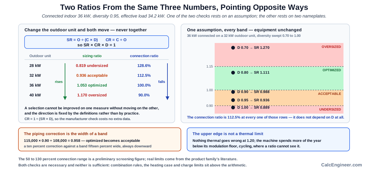
The two ratios are not independent, and the relationship between them is a matter of algebra rather than of engineering practice.

Write the definitions the page uses:

SR = O / (C × D)      sizing ratio
CR = C / O            connection ratio

O   outdoor unit rated capacity, BTU/h or kW
C   connected indoor nameplate total, BTU/h or kW
D   diversity factor, dimensionless, 0.0 to 1.0

Multiply them together and the two capacities cancel:

SR × CR = [O / (C × D)] × [C / O] = 1 / D

and therefore

SR × CR × D = 1

The three examples on the page satisfy it, as they must:

Imperial:         1.065 × 1.043 × 0.90 = 1.000
Metric:           0.936 × 1.125 × 0.95 = 1.000
Page text worked: 1.059 × 1.111 × 0.85 = 1.000

What the identity says:

The three quantities are locked together, so fixing any two
fixes the third.
At a given diversity factor the sizing ratio and the connection
ratio are inversely proportional to one another.
Enlarging the outdoor unit raises the first and lowers the
second, by the same factor.

What it does not say:

It is not an industry rule and it expresses no physical law.
It follows from the two definitions in use on this page, and it
would take a different form under different definitions. Some
manufacturers define a combination ratio on a diversified basis
rather than a nameplate one, and the algebra then changes with
it.

What follows from it in practice is the useful part:

The connection ratio can be obtained from quantities already
entered:

  CR = 1 / (SR × D)

with no further data required. The manufacturer limit can
therefore be checked at the screening stage without opening the
manufacturer's literature, even though the limit itself has to
come from that literature.

Per the definitions used by the calculator: the sizing ratio and the connection ratio share their terms, and the product of the two with the diversity factor equals unity, which is an algebraic consequence of how the two are defined rather than a rule of practice.

Where the Two Ratios Collide

Rearranging the identity exposes a region in which a selection sits inside the calculator's preferred band and outside a manufacturer connection limit at the same time.

Start from the rearranged form. If the permitted connection ratio has an upper limit CR_max, then:

CR = 1 / (SR × D) ≤ CR_max

  →  SR_min = 1 / (CR_max × D)

Against the preliminary screening figure of 130 percent the page names, that gives:

D = 0.70 → SR_min = 1.099
D = 0.75 → SR_min = 1.026
D = 0.80 → SR_min = 0.962
D = 0.85 → SR_min = 0.905
D = 0.90 → SR_min = 0.855
D = 1.00 → SR_min = 0.769

The optimized band starts at 1.00, and that is where the two meet:

Below a diversity factor of 0.769 the minimum permissible
sizing ratio rises above unity, and the lower part of the
optimized band becomes unreachable.
At a diversity of 0.70 everything below 1.099 is out of reach,
which is two thirds of a band 0.15 wide.

A case in numbers:

Connected indoor total 100 kW (341,200 BTU/h),
diversity factor 0.70:

  Effective load:   70 kW (238,850 BTU/h)
  Outdoor unit 70 kW (238,850 BTU/h): SR = 1.00 → OPTIMIZED
  Connection ratio: 100 / 70 = 143 percent

The connection ratio exceeds the preliminary screening figure of
130 percent while the sizing ratio sits exactly on the lower
edge of the band the page calls optimal.

A solution exists, and it is worth seeing where it lies:

An outdoor unit of at least 100 / 1.30 = 76.9 kW (262,400 BTU/h)
gives a connection ratio of exactly 130 percent and a sizing
ratio of 76.9 / 70 = 1.099, which is still inside the optimized
band.
The band is not lost, but only its upper third remains
available.

The limit itself needs stating carefully:

The 130 percent figure is carried by the page as a preliminary
screening range, not as a universal constraint. Actual limits
depend on the manufacturer, the product family, the particular
outdoor unit, the combination of indoor units and the operating
conditions, and they are verified against the manufacturer's
documentation.
What the arithmetic above shows is the shape of the dependence,
not a set of permissible combinations.

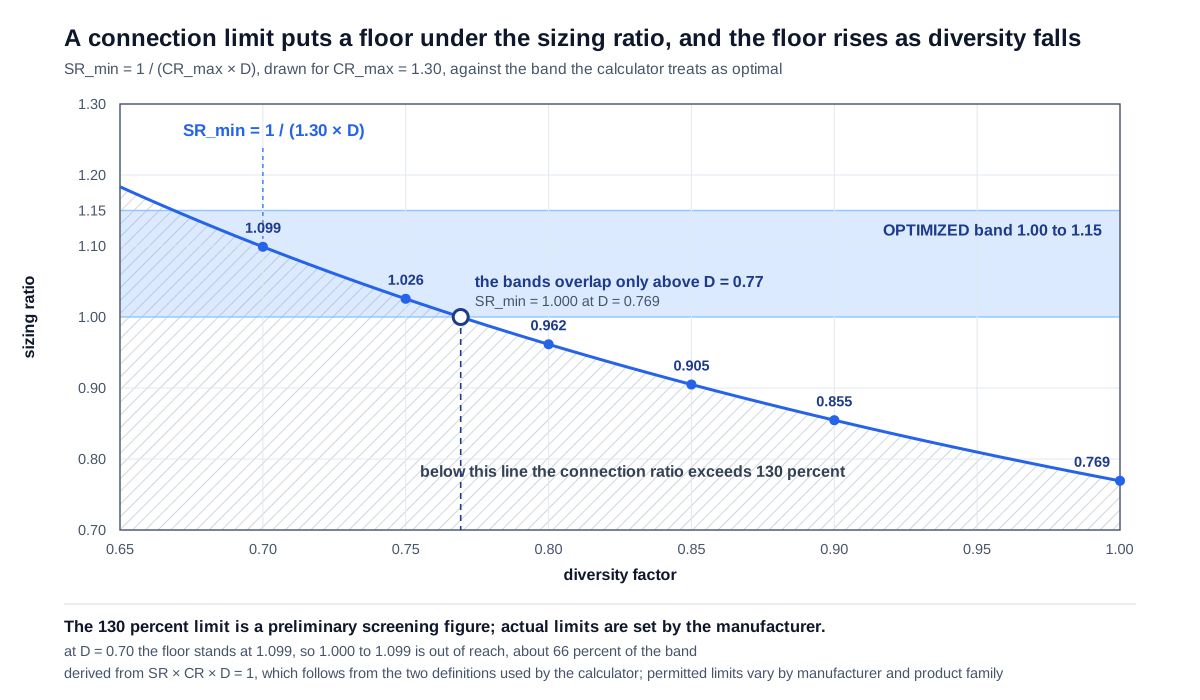
Per the definitions used by the calculator and manufacturer connection ratio practice: rearranging the identity gives a minimum sizing ratio for any stated connection limit, and at low diversity that minimum rises above the lower edge of the band the calculator treats as optimal.

Reading the Bands Against a Connection Limit

The classification bands and the connection limit answer different questions, and a selection has to satisfy both without either standing in for the other.

What each measure assesses:

The sizing ratio asks whether the outdoor unit can meet the
simultaneous load expected of it.
The connection ratio asks whether the manufacturer permits that
set of indoor units on that outdoor unit at all.

Why one does not substitute for the other:

The connection limit is a property of the system architecture:
the number and total capacity of indoor units the outdoor unit
can serve on its refrigerant circuit, its oil return behaviour
and its charge. It is not a statement about the thermal balance.
The sizing ratio is a statement about load and nothing else.
A system can satisfy either one and violate the other, in both
directions.

The reverse case is easy to miss, because it looks like an error:

The lower connection limit, given as 50 percent, corresponds to
a sizing ratio of

  SR = 1 / (0.50 × D)

which at a diversity factor of 0.90 is 2.22. The calculator
places that in its upper oversized band, while the connection
check passes it without comment.

What such a combination represents:

A small number of indoor units on a large outdoor unit.
That is a normal condition on a phased fit-out, where the rest
of the indoor units are connected in a later tranche, and the
high sizing ratio then records reserve capacity rather than a
mistake.
It is also what a landlord's base build looks like before the
tenancies are taken.

How to read the returned category:

As one of two checks rather than as a conclusion. The category
describes the match to load under an assumed diversity factor,
and says nothing about whether the combination is permitted.

Per manufacturer combination practice and the calculator's stated scope: the connection limit constrains which combinations of units are permitted, while the sizing ratio addresses whether the outdoor unit meets the expected load, and a selection has to satisfy both.

Nameplate Capacity Is Not Delivered Capacity

The outdoor capacity entered into the calculation is a rating at standard conditions, and what reaches the indoor units after the refrigerant has travelled through the pipework is less than that.

What reduces it:

Equivalent pipe length, which includes the local losses of
branch joints, headers and bends as well as the measured run.
Elevation difference between the outdoor unit and the indoor
units, where the sign of the difference matters and the
permitted values differ for outdoor unit above and below.
The number of connected indoor units and how they are
distributed across the branches.

The order of magnitude:

Manufacturer engineering data gives correction factors as
tables or curves against equivalent length. Reductions on the
order of ten percent appear in published data for long runs,
and the figure for any given system depends on the product
family and has to be read from that manufacturer's tables.

What that does to the returned ratio, using the page example:

The sizing ratio is computed on the nameplate figure. Correcting
the outdoor capacity down by ten percent gives

  115,000 × 0.90 = 103,500 BTU/h (30.3 kW)
  103,500 / 108,000 = 0.958

which moves the result from OPTIMIZED to ACCEPTABLE. A fifteen
percent correction gives 97,750 BTU/h (28.6 kW) and a ratio of
0.905, still ACCEPTABLE but close to the bottom of that band.

Why this matters more than it first appears:

The optimized band is fifteen percent wide, which is the same
order as the piping correction itself.
A selection landing in the middle of the band on nameplate
figures can sit at its edge in service, and the movement is
always in the same direction.

What is done about it in practice:

Enter the corrected outdoor capacity rather than the nameplate
figure, where the route is known well enough at the screening
stage to read a correction factor.
Or carry margin deliberately at the screening stage and settle
the question in the manufacturer's selection software, which
applies the corrections for the actual pipe network.

Per manufacturer engineering data for variable refrigerant flow systems: rated outdoor capacity is corrected for equivalent pipe length and elevation difference, and the correction is comparable in magnitude to the width of the classification band.

Heating May Select a Different Machine

The calculation addresses cooling, and in a heating-dominated climate the outdoor unit that satisfies the cooling ratio may not satisfy the heating requirement.

What changes in heating:

Heat pump capacity falls as outdoor temperature falls, because
the suction vapour becomes less dense and the pressure ratio
across the compressor rises.
Defrost interrupts heat delivery periodically, which reduces
the average capacity over a period below the steady figure.

What that means for selection:

Rated heating capacity is published at a stated outdoor
condition. At the winter design temperature for the site the
available capacity can be substantially lower.
An outdoor unit giving a cooling sizing ratio inside the
optimized band can be short of the heating requirement at the
same time, on the same building.

How the conflict is resolved:

Run the calculation for both modes and take the larger of the
two required sizes.
Or provide supplementary heat from another source for the
coldest hours, which allows the outdoor unit to be selected on
cooling and keeps the machine out of its least efficient
operating region.

What complicates the comparison:

The diversity factor for heating need not equal the one for
cooling. Zones that require cooling in summer because of solar
gain may require less heat in winter for the same reason, so
the coincident peak has a different shape in the two modes.
Heat recovery systems move heat between zones that are calling
for cooling and heating at once, which changes the problem
statement rather than the number.

What the page says about it:

The page states that it evaluates the ratio for the cooling
mode and that heating operation requires separate verification.

Per manufacturer engineering data and ASHRAE Handbook, HVAC Systems and Equipment: heat pump capacity falls with outdoor temperature and is further reduced by defrost, so a heating design condition can select a larger outdoor unit than the cooling ratio requires.

Oversizing Costs More Than Money Here

The usual penalty for an oversized machine is first cost, and a variable refrigerant flow system adds a second penalty at the bottom of its operating range.

What happens at low load:

A variable speed compressor reduces capacity down to a minimum,
below which it cannot modulate further and has to cycle on and
off instead.
That minimum stable capacity is a fraction of nominal capacity
and the fraction differs between product families.

Why surplus size makes it worse:

The larger the outdoor unit relative to the load, the more of
the year the system spends below its own minimum and cycling.
The advantage of modulation is then lost in precisely the
region where it is worth most, because a VRF system spends the
large majority of its operating hours at part load rather than
at design load.

What that does to energy use:

The rating figures published for multi-split systems are
weighted for part load operation, and they carry an assumption
that the equipment is inside its modulation range while
operating there.
Equipment that falls out of the bottom of that range does not
reach the rated figures, and the shortfall does not appear
anywhere in a capacity ratio.

What the page says:

It notes that oversizing raises first cost without a
proportional gain in flexibility or efficiency.

How that connects to the bands:

The optimized band is bounded above at 1.15, and that upper
edge reflects this consideration rather than a thermal
calculation. Nothing thermal goes wrong at 1.20; what goes
wrong is the fraction of the year spent below the modulation
floor.

Per ASHRAE Handbook, HVAC Systems and Equipment, on variable capacity equipment: performance at part load depends on the compressor remaining within its modulation range, and an oversized outdoor unit spends more of its operating hours below that range.

Combination Rules Sit Above the Arithmetic

Two selections with identical ratios can differ in whether the manufacturer permits them at all, because permission depends on which units are connected rather than on how much they add up to.

What the combination rules fix:

Which indoor and outdoor models may be paired within a product
family.
The maximum number of indoor units on one outdoor unit and on
one branch.
The branch fittings and headers required, and where they may be
placed along the route.
Limits on mixing indoor unit sizes and types on the same
circuit.

Why a ratio cannot carry this:

The connected total is a sum, and the same sum arises from
quite different schedules.
Twenty small indoor units and five large ones can total the
same capacity and differ in whether the combination is
permitted.

What else constrains the same selection:

The pipe length from the outdoor unit to the furthest indoor
unit, and the total length of the whole network.
The elevation difference between the highest and lowest indoor
units.
Refrigerant charge limits, including the concentration
permitted on a leak into the smallest occupied space served,
which is a safety requirement rather than a performance one.

What follows:

The sizing ratio is a necessary condition and not a sufficient
one.
The sufficient check is made in the manufacturer's selection
software against the actual schedule of equipment and the
actual pipe network.

Per manufacturer combination tables and selection software practice: permitted configurations depend on the specific units connected, on the pipe network and on refrigerant charge limits, none of which follow from the capacity sum alone.

What a Ratio Cannot See

A dimensionless number carries no information about what produced it, and two selections with the same ratio can face quite different circumstances.

What is discarded in forming the ratio:

The absolute size of the system. A ratio of 1.05 reads the same
on a 20 kW (68,200 BTU/h) system and a 200 kW (682,400 BTU/h)
one.
The schedule of indoor units.
The number of zones and how they are distributed through the
building.

Why absolute size matters here:

Outdoor unit capacities are available in discrete steps, and
the step is a large fraction of a small system and a small
fraction of a large one.
Whether a narrow band can be hit at all therefore depends on
the size of the system.

The arithmetic of that:

At an effective load of 20 kW (68,200 BTU/h) with steps of 2 kW
(6,800 BTU/h), adjacent candidates give ratios of 1.00 and
1.10, and both sit inside the optimized band.

At an effective load of 8 kW (27,300 BTU/h) with the same 2 kW
step, adjacent candidates give 1.00 and 1.25, and the second
falls outside it.

What follows from that:

On a small system, landing in the band is decided by whether a
suitable size exists in the range, not by the quality of the
load calculation.
The returned category then reports the manufacturer's product
range as much as the design decision, and refining the load
estimate will not move it.

Per manufacturer product range practice: outdoor unit capacities are available in discrete steps, and the step is a larger fraction of a small system than of a large one, so the achievable sizing ratio depends on the size of the system as well as on the load.

Worked Example: 115,000 Against an Effective 108,000

The imperial example on the page, carried further than the page carries it.

Connected indoor capacity   120,000 BTU/h (35.2 kW)
Diversity factor            0.90
Outdoor unit capacity       115,000 BTU/h (33.7 kW)

Step 1, the effective load.

120,000 × 0.90 = 108,000 BTU/h (31.7 kW)

Step 2, the sizing ratio.

115,000 / 108,000 = 1.065

Step 3, the classification.

1.065 lies between 1.00 and 1.15 → OPTIMIZED

Step 4, the connection ratio, obtained two ways.

From the identity: CR = 1 / (SR × D) = 1 / (1.065 × 0.90) = 1.043
Direct:            CR = 120,000 / 115,000 = 1.043

The agreement is the identity being satisfied rather than a
coincidence. The value is 104.3 percent, inside the preliminary
screening range of 50 to 130 percent.

Step 5, the margin to the connection limit.

At a limit of 130 percent the smallest permissible outdoor unit
is 120,000 / 1.30 = 92,300 BTU/h (27.0 kW), which corresponds to
a sizing ratio of 92,300 / 108,000 = 0.855.
The selection stands well clear of that limit, and the whole of
the optimized band is available on this diversity assumption.

Step 6, sensitivity to the diversity factor.

Same equipment, different assumption:

  D = 0.80: effective 96,000 BTU/h (28.1 kW), SR = 1.198 → OVERSIZED
  D = 0.90: effective 108,000 BTU/h (31.7 kW), SR = 1.065 → OPTIMIZED
  D = 1.00: effective 120,000 BTU/h (35.2 kW), SR = 0.958 → ACCEPTABLE

The category changes twice while the equipment does not change
at all.

Step 7, what the piping correction does.

Correcting the rated outdoor capacity down by ten percent:

  115,000 × 0.90 / 108,000 = 0.958 → ACCEPTABLE

The correction is comparable to the width of the band, so it
moves the result across a band boundary on its own.

Step 8, what the position within the band is worth.

A value of 1.065 stands 6.5 percent above the lower edge of the
band and 8.0 percent below the upper one, which is close to the
middle.
That position leaves room for the piping correction in one
direction and for a revision of the diversity assumption in the
other, which is the practical reason for preferring the middle
of a band to its edges.

Step 9, what the check does not cover.

The combination rules for the actual schedule of indoor units.
The heating design case.
Whether a 115,000 BTU/h (33.7 kW) size exists in the chosen
product family at all.

Step 10, what follows.

Check the connection ratio against the limit published for the
selected product family rather than against the preliminary
screening figure.
Correct the outdoor capacity for equivalent pipe length and
elevation where the route is known.
Confirm the whole selection in the manufacturer's software.

Metric Example and the Diversity Sweep

The metric example on the page starts closer to a boundary, which makes it the more useful of the two for showing how far the answer travels.

Connected indoor capacity   36 kW (122,800 BTU/h)
Diversity factor            0.95
Outdoor unit capacity       32 kW (109,200 BTU/h)

Effective load: 36 × 0.95 = 34.2 kW (116,700 BTU/h)
Sizing ratio:   32 / 34.2 = 0.936 → ACCEPTABLE

The connection ratio for the same selection:

36 / 32 = 1.125, that is 112.5 percent
Identity check: 0.936 × 1.125 × 0.95 = 1.000

What the pair of values says together:

The sizing ratio is below unity, so the outdoor unit is smaller
than the assumed simultaneous load.
The connection ratio sits inside the preliminary screening
range.
Both checks pass, but the first passes with very little margin,
and it is the one resting on an assumption.

What the next size up does:

An outdoor unit of 36 kW (122,800 BTU/h) gives a sizing ratio of
36 / 34.2 = 1.053 → OPTIMIZED, and a connection ratio of exactly
100 percent.
One step in the product range moves the result across a band
boundary.

Sweeping the diversity factor across the range the page calls typical, with the equipment held at 36 kW connected and a 32 kW outdoor unit:

D = 0.70: effective 25.2 kW (86,000 BTU/h),  SR = 1.270 → OVERSIZED
D = 0.80: effective 28.8 kW (98,270 BTU/h),  SR = 1.111 → OPTIMIZED
D = 0.90: effective 32.4 kW (110,550 BTU/h), SR = 0.988 → ACCEPTABLE
D = 0.95: effective 34.2 kW (116,700 BTU/h), SR = 0.936 → ACCEPTABLE
D = 1.00: effective 36.0 kW (122,800 BTU/h), SR = 0.889 → UNDERSIZED

What the sweep shows:

The same equipment passes through all four categories as the
diversity factor moves across the range the page describes as
typical.
The quantity the engineer selects by judgement therefore
determines the verdict completely, and no property of the
equipment changed anywhere in that table.

What the connection ratio does over the same sweep:

It stays at 112.5 percent throughout, because it does not
depend on the diversity factor at all.
That is the substantive difference between the two checks: one
rests on an assumption and the other rests on two nameplate
figures.

Per the definitions used by the calculator: the connection ratio depends only on the two nameplate quantities while the sizing ratio depends additionally on an assumed diversity factor, so the two checks differ in how much of the result rests on judgement.

Application Boundaries: Selection, Piping, Verification

The model applies to the ratio of outdoor unit rated capacity to the effective load under an assumed diversity factor, in cooling, on nameplate figures. The following require separate treatment.

The diversity factor. A design assumption, not a measurement. Moving it across the range the page calls typical, 0.70 to 0.95, carries the same equipment through every category, as the sweep above shows. An hourly load calculation returning the coincident peak is the stronger basis.

The connection ratio. It follows from the same quantities as CR = 1 / (SR × D) and is checked against the limit published for the selected product family, not against the 50 to 130 percent preliminary screening range.

Combination rules. These depend on the schedule of indoor units rather than on the sum of their capacities, so two selections with identical ratios can differ in whether they are permitted.

Piping corrections. Equivalent length and elevation difference reduce available capacity by an amount comparable to the width of a classification band, roughly ten percent on long runs in published data, always in the same direction.

The heating design case. Capacity falls with outdoor temperature and is further reduced by defrost, so heating can select a larger size than cooling does, and the two diversity assumptions need not be equal.

Refrigerant charge limits. The charge in the circuit is bounded by the concentration permitted on a leak into the smallest occupied space served, which is a safety constraint independent of everything above.

Discrete product sizes. Whether the band can be hit depends on what exists in the range, and on a small system that consideration dominates the accuracy of the load estimate.

Part load behaviour. Minimum stable capacity and cycling below it do not appear in a capacity ratio, and they are where an oversized machine actually costs money.

Final selection. Made in the manufacturer's selection software against the actual schedule of equipment and the actual pipe layout.

Per the calculator's stated scope and manufacturer selection practice: a capacity ratio on an assumed diversity basis is the scope of this model, while the diversity assumption itself, connection limits, combination rules, piping corrections, the heating case and refrigerant limits each require separate treatment.

VRF System Sizing Calculator

Standards and References

• ASHRAE Handbook, HVAC Systems and Equipment (American Society of Heating, Refrigerating and Air-Conditioning Engineers, current edition), chapter on variable refrigerant flow systems. System architecture, part load operation, and the behaviour of variable capacity equipment as outdoor conditions change.
• ASHRAE Handbook, Fundamentals (American Society of Heating, Refrigerating and Air-Conditioning Engineers, current edition). Cooling and heating load calculation, and the coincident peak from which a diversity factor is derived.
• AHRI Standard 1230, Performance Rating of Variable Refrigerant Flow (VRF) Multi-Split Air-Conditioning and Heat Pump Equipment (Air-Conditioning, Heating, and Refrigeration Institute, current edition). The rating conditions at which the nameplate capacities used in both ratios are published.
• ANSI/ASHRAE/IES Standard 90.1, Energy Standard for Sites and Buildings Except Low-Rise Residential Buildings (current edition). Minimum equipment efficiency requirements and the part load metrics applied to multi-split equipment.
• ASHRAE Standard 15, Safety Standard for Refrigeration Systems (current edition). Refrigerant concentration limits for the occupied space served, which bound the charge a circuit may carry.
• Manufacturer engineering data for variable refrigerant flow systems (current published editions). Combination rules, connection ratio limits by product family, correction factors for equivalent pipe length and elevation difference, and minimum stable capacity.
• Manufacturer selection software (current released versions). Verification of a proposed combination against the actual schedule of indoor units and the actual pipe network, which is where a screening result is confirmed or rejected.
• Published work on the energy performance of multi-split systems (current editions of the building energy literature). Part load behaviour, measured performance against rated figures, and the effect of surplus capacity on achieved efficiency.

FAQ

Related Calculators

• Cooling Load Calculator: the room loads whose sum sets the connected indoor capacity, and the place where an hourly result would give the coincident peak directly rather than through an assumed diversity factor.
• HVAC Heat Load Calculator: envelope gains zone by zone, which is what has to exist before a coincident peak can be worked out for a multi-zone building.
• AC Tonnage Calculator: conversion of a load into refrigeration capacity, useful when comparing an effective load against the discrete sizes a product range offers.
• Heat Pump Size Calculator: sizing on the heating design case, which for a VRF system is checked separately from cooling and can select the larger machine.
• Chiller Capacity Calculator: the alternative central plant arrangement, where diversity enters through the water side and the connection limit has no counterpart.
• Psychrometric Calculator: the air state behind the split of a zone load into sensible and latent parts, which is what decides the indoor unit selection that forms the connected total.
• CFM Calculator: the airflow an indoor unit needs to deliver its share of the load, checked once the indoor schedule is fixed.
• Cooling Tower Calculator: heat rejection for water-cooled arrangements, which some VRF product families use in place of air-cooled outdoor units.