Velocity Pressure: The Square Root That Halves the Error, and the Square That Puts It Back

One Field, One Line, and a Constant Carrying a Density

Moving air carries kinetic energy. Bringing it to rest against an opening that faces into the flow converts that energy into a rise in pressure, and the size of the rise is the velocity pressure. The relation between it and the speed of the air is one line of fluid mechanics, and in HVAC practice that line is written with a number in it. Divide the velocity by 4005, square the result, and the answer is the pressure in inches of water column.

The calculation is a single squaring of a single number. Everything worth knowing about it is inside the constant and outside the arithmetic.

That constant is not a unit conversion alone. It carries an assumption about the density of the air, and the assumption is standard sea level air at ordinary temperature. Air at reduced barometric pressure or elevated temperature is lighter, produces less pressure at the same speed, and the constant then reports a speed lower than the one actually present. Nothing on the page announces this, because the density has been absorbed into a number that looks like a pure unit factor.

The same relation is the basis of the commonest field measurement of airflow in a duct, and running it backwards is where its behaviour becomes interesting. Because velocity comes out of pressure through a square root, a given percentage error in the pressure becomes half that percentage in the velocity, which is a favourable property and holds at every speed. Because pressure falls with the square of velocity, an instrument that resolves a fixed smallest increment sees that increment become a larger and larger fraction of the reading as the air slows. The two effects work against each other, and which one dominates depends on where in the range the measurement sits.

What follows works out where the constant comes from, what it becomes at other densities, how the two opposing effects on accuracy combine, and where the balance between them shifts far enough to change which instrument is appropriate. The calculator takes a velocity and returns a pressure. The field work runs the other way, and that direction is where the difficulties are.

Calculator Inputs: A Velocity In, Three Units Out

The field list is one entry long, and the shortness is worth dwelling on, because everything else in the model has been decided in advance.

Air Velocity   FPM in imperial mode, m/s in metric mode
               accepted range 100 to 6,000 FPM
               (0.5 to 30.5 m/s)

That goes into one relation:

VP = (V / 4005)²

V    air velocity, feet per minute
       typical duct values run from about 400 FPM
       (2.0 m/s) in branches to about 2,500 FPM
       (12.7 m/s) in mains
VP   velocity pressure, inches of water column
       typical values from 0.010 to 0.39 in.w.c.
       (2.5 to 97 Pa) across that velocity range

A metric entry is converted to feet per minute before the relation is applied, so both unit systems run the same arithmetic and return the same pressure.

The result comes back in three units: velocity pressure in inches of water column, in pascals and in pounds per square inch. The conversions the page carries between them are these.

1 in.w.c. = 249.089 Pa = 0.0361 psi
1 psi     = 6,894.76 Pa = 27.68 in.w.c.

The single field points in one direction only. The calculator runs from a known velocity to a pressure, while field work runs the other way: a manometer shows a pressure, and a velocity is derived from it. The inverse relation is V = 4005 √VP, and the two directions differ in how they carry uncertainty.

What the field list does not contain is the more informative half of the problem. Air density, which the constant assumes to be standard. Temperature and barometric pressure, which together determine that density, and which the Air Density Calculator turns into a figure. Cross-sectional area, which is needed to reach an airflow. Each of those is worked out below, or identified as belonging to a separate step.

Three Pressures and What the Instrument Actually Reads

A duct carries three pressures that share a name and differ in what they describe, and the instrument used to measure the third of them reads none of the three directly.

Static pressure acts in all directions and represents the potential component, picked up by an opening set flush with the duct wall, parallel to the flow. Velocity pressure acts in the direction of motion and represents the kinetic component. Total pressure is the sum of the two, and is picked up by an opening facing into the flow.

TP = SP + VP,   so   VP = TP − SP

A Pitot-static tube is built to give that difference without measuring either term on its own. It carries two channels: a central one facing into the flow, which senses total pressure, and a ring of side holes, which sense static pressure. Both are connected to opposite sides of a manometer, and the instrument shows their difference, which is the velocity pressure. Neither the total nor the static pressure is read separately in that arrangement.

Reading a difference has a consequence for accuracy that the arithmetic makes plain. Each of the two quantities being differenced is substantially larger than the difference itself. With a static pressure of 1.0 in.w.c. (249 Pa) and a velocity pressure of a few hundredths, the instrument is resolving a small difference between two large numbers, and the uncertainty of the difference draws on both channels.

Two field conditions degrade that difference further. Misalignment of the tube with the flow reduces the total pressure sensed at the facing opening, and swirl downstream of an elbow or a branch makes the static holes sensitive to the cross-stream component of velocity. Both are why straight duct is required upstream and downstream of the measuring point.

Per ANSI/ASHRAE Standard 111-2024 and ASHRAE Handbook, Fundamentals: a Pitot-static tube presents total pressure to one port and static pressure to the other, so the manometer reads their difference, which is the velocity pressure, and the accuracy of that difference depends on both channels.

Where 4005 Comes From

The constant is the general relation with a density substituted into it. Reconstructing it shows exactly which density, and the answer is not quite the one usually quoted alongside it.

The general form:

VP = ½ × ρ × V²

VP   dynamic pressure, pascals
ρ    air density, kilograms per cubic metre
       standard reference values run 1.20 to 1.29 kg/m³
       (0.075 to 0.080 lb/ft³) over ordinary conditions
V    velocity, metres per second

That form requires consistent units. Substituting quantities in other units returns a result in other units, and folding those conversions into a single number is what produces a constant.

Moving to the imperial statement means converting both quantities:

Velocity, feet per minute to metres per second:
  V[m/s] = V[fpm] × 0.00508
Pressure, pascals to inches of water column:
  divide by 249.089

VP[in.w.c.] = ½ × ρ × (0.00508 × V)² / 249.089

Substituting the rounded density gives a coefficient:

At ρ = 1.2 kg/m³ (0.0749 lb/ft³):
  ½ × 1.2 × 0.00508² / 249.089 = 6.216 × 10⁻⁸

The relation becomes VP = 6.216 × 10⁻⁸ × V², which is equivalent to a divisor of about 4010. Working backwards from the published constant gives the density it actually carries: the coefficient behind (V / 4005)² is 6.234 × 10⁻⁸, which corresponds to a density of about 1.204 kg/m³ or 0.0751 lb/ft³.

The rounded reference values 1.2 and 0.075 quoted alongside the constant are correct as reference points, but they do not reproduce 4005 exactly on substitution. The gap is about three tenths of a percent, and it comes from roundings accumulated in the derivation. For field measurement it is not significant.

Three separate things are inside that one number: the factor of one half from the general relation, the conversion of velocity from feet per minute to metres per second, and the conversion of pressure from pascals to inches of water column. All three are folded together, which is why the result looks arbitrary. It also means the constant is valid at the density built into it, and nowhere else without adjustment.

Per ASHRAE Handbook, Fundamentals, on fluid flow: the imperial constant is the general dynamic pressure relation with standard air density and the unit conversions folded into a single number, and reconstructing it identifies the density it assumes as about 1.204 kg/m³.

The Constant Moves With Density

Lighter air produces less pressure at the same speed. A reading taken in air of reduced density and interpreted with the standard constant therefore reports a velocity lower than the one actually present, and the size of that understatement follows from the relation directly. From VP = ½ρV² comes V = √(2 VP / ρ), so velocity varies inversely with the square root of density, and the constant scales the same way.

C = 4005 × √(ρ_std / ρ_actual)

with density in lb/ft³ and ρ_std = 0.075:
  C = 4005 × √(0.075 / ρ)

Three worked values:

ρ = 0.075 lb/ft³ (1.201 kg/m³):   C = 4005
ρ = 0.0625 lb/ft³ (1.001 kg/m³):  C = 4387
ρ = 0.0602 lb/ft³ (0.964 kg/m³):  C = 4470

Densities below the standard value arise at reduced barometric pressure, at elevated air temperature, or from a combination of the two. The actual figure follows from both parameters together and is calculated for the conditions at the measuring point rather than assigned from either one alone.

Using the tabulated constant instead costs something at each of those densities. At 0.0625 lb/ft³ (1.001 kg/m³), a velocity computed with 4005 is understated in the ratio 4005/4387, which is 8.7 percent low taking the corrected velocity as the base. At 0.0602 lb/ft³ (0.964 kg/m³), the understatement is 10.4 percent on the same basis.

The error does not stay in the velocity. Airflow is velocity times area, so an understated velocity carries into it in full, and balancing a system in air of reduced density with the standard constant understates every computed airflow by the same percentage.

There are two ways to handle it in the field, and they start from the same step. Determine the density from the barometric pressure and the temperature at the measuring point, then either correct the constant with the relation above or work in the general ½ρV² form throughout.

One distinction matters here and is easy to lose. This correction applies to the density at the point of measurement. Correcting a measured airflow to standard conditions for comparison against a fan curve is a different operation with a different purpose, and the two are not interchangeable.

Per ASHRAE Handbook, Fundamentals, and AMCA Publication 203: the velocity constant scales with the square root of the density ratio, so applying the standard value in air of lower density understates the velocity derived from a given pressure reading.

The Square Root Cuts the Error in Half, and the Manometer Puts It Back

Two properties of the same one-line relation act on accuracy in opposite directions. Where they balance decides which instrument suits a given measurement, and the balance point is arithmetic rather than physics.

The property working in favour is the square root itself. Velocity is recovered by taking a square root, so relative uncertainty is halved in the process.

V ∝ √VP   →   ΔV/V = ½ × ΔVP/VP

A ten percent uncertainty in the pressure gives five percent in the velocity, and that holds at every speed.

The property working against it is the squaring. Pressure falls with the square of velocity, while the smallest increment an instrument can resolve is an absolute quantity that does not fall at all. Halve the velocity and the pressure drops to a quarter, so the same absolute resolution becomes four times the fraction of the reading.

The numbers, at an assumed resolution of 0.005 in.w.c. (1.25 Pa):

   V, fpm     V, m/s   VP, in.w.c.    VP, Pa   pressure   velocity
      500       2.54       0.0156       3.88     32.1%      16.0%
      600       3.05       0.0224       5.59     22.3%      11.1%
      800       4.06       0.0399       9.94     12.5%       6.3%
    1,000       5.08       0.0623      15.53      8.0%       4.0%
    1,500       7.62       0.1403      34.94      3.6%       1.8%
    2,000      10.16       0.2494      62.12      2.0%       1.0%
    3,000      15.24       0.5611     139.76      0.9%       0.45%

The resolution used here is taken as characteristic of an inclined mechanical manometer. Digital instruments resolve differently, to a figure their manufacturer publishes, and the table is recomputed for whatever that figure is.

Taking five percent as an acceptable uncertainty in the velocity, the condition is satisfied once the pressure is large enough.

VP ≥ 0.005 / (2 × 0.05) = 0.05 in.w.c. (12.5 Pa)
V  = 4005 × √0.05 = 896 FPM (4.55 m/s)

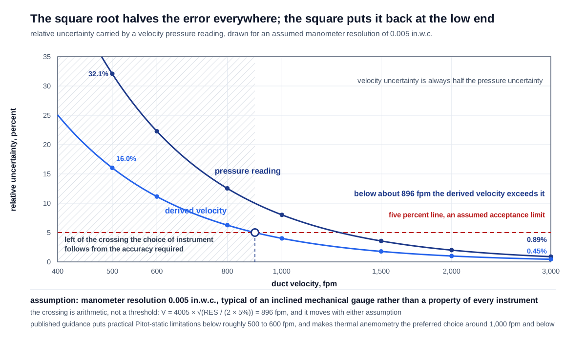
That 896 FPM figure is the result of an assumed instrument resolution and an assumed acceptance limit, and it moves whenever either assumption moves. It is not a point at which the method stops working. Published guidance places the practical limitations of a Pitot-static tube below roughly 500 to 600 FPM (2.5 to 3.0 m/s), while thermal anemometry becomes the preferred choice around 1,000 FPM (5.1 m/s) and below. Between those figures lies a region in which the choice of instrument follows from the accuracy required and the conditions at the point, not from either method failing.

Per instrument manufacturer data and ANSI/ASHRAE Standard 111-2024: the square root relation halves the relative uncertainty carried from pressure into velocity, while the quadratic fall of pressure with velocity raises the relative weight of a fixed instrument resolution, and the balance between the two shifts with velocity rather than breaking at a threshold.

Where the Thermal Method Takes Over

The alternative at low velocity does not measure pressure at all, which is the whole reason its sensitivity holds up where a pressure reading loses precision.

The move from one method to the other is gradual and is decided by the accuracy required, not by a sharp boundary. A thermal anemometer measures no pressure, so the quadratic fall that erodes a Pitot reading does not apply to it.

The instrument works on a heat balance. A heated element is placed in the flow, and the rate at which heat leaves it depends on the speed of the air passing over. The instrument either holds the element at constant temperature and measures the power needed to do so, or supplies constant power and measures the temperature reached. Velocity follows from that balance rather than from a pressure.

That is what helps at the low end. Convective heat transfer varies roughly with the square root of velocity in the low range, rather than with its square, so sensitivity falls away far more slowly as the air slows, which is the opposite of the behaviour described in the previous section.

Something is given up in exchange. The reading depends on the temperature and density of the medium, so the instrument needs correction or built-in compensation. Flow direction is not resolved, because the sensor responds to the magnitude of the velocity. And contamination of the sensing element changes its heat transfer and shifts the reading.

Each method has its place. Pitot-static in mains, at higher velocities, in dirty airstreams and wherever robustness matters more than resolution. Thermal anemometry in branches, at outlets, at low velocities and in clean air.

A third approach sidesteps the question altogether. A flow hood placed over a diffuser or grille captures the whole outlet and measures the volume passing through it, avoiding the question of how velocity is distributed across a section.

Per ANSI/ASHRAE Standard 111-2024 and NEBB procedural practice: thermal anemometry derives velocity from convective heat transfer rather than from pressure, so its sensitivity does not collapse as velocity falls, at the cost of dependence on air temperature and on the cleanliness of the sensing element.

From a Reading to an Airflow

The pressure reading is two steps away from the quantity actually wanted, and each step adds uncertainty of its own kind.

VP  →  V = 4005 √VP  →  Q = V × A

VP   measured velocity pressure, in.w.c. (Pa)
V    velocity at the measuring point, FPM (m/s)
A    cross-sectional area, ft² (m²)
Q    volumetric airflow, CFM (m³/h)

The first step halves the relative uncertainty of the pressure and adds the uncertainty of the assumed density. The second adds the uncertainty of the area and, more importantly, the assumption that the measured velocity represents the average across the section. That second step is the one the CFM Calculator carries out once the velocity and the area are known.

One point is not enough for it. Velocity is not uniform across a duct: it falls to zero at the walls and exceeds the average near the centre. A single-point reading returns a value different from the average, and the direction of the difference depends on where the point sits. The traverse procedure, which samples a defined grid of points, is set out in the companion article on calculating air velocity in duct design and is not repeated here.

The chain in numbers runs as follows. At a measured 0.0898 in.w.c. (22.36 Pa) with a resolution of 0.005 in.w.c. (1.25 Pa), the pressure uncertainty is 5.6 percent and the velocity uncertainty is 2.8 percent. With a two percent uncertainty in the area, the airflow uncertainty is about 3.4 percent when the two are combined independently. The uncertainty contributed by an incomplete traverse adds to that, and under favourable conditions it is comparable in size to the terms already listed.

What follows from that arithmetic is a limit on what can be claimed. A field accuracy of about five percent on a duct airflow is reachable at high velocity, with a full traverse and a known density. It is not reachable when any one of those three conditions is relaxed.

Per ANSI/ASHRAE Standard 111-2024 and NEBB Procedural Standards: deriving an airflow from a velocity pressure reading passes through velocity and area, and the traverse assumption that the sampled velocities represent the section contributes an uncertainty comparable to the instrument itself.

Velocity Pressure Is Not Lost, It Is Converted

The three pressures exchange with one another along a duct. Knowing which of them changes where explains behaviour that otherwise reads as a contradiction.

Along a section carrying no fan, total pressure falls in the direction of flow, because friction and turbulence convert energy irreversibly into heat. Across a fan, total pressure rises: the fan adds energy to the stream, and that addition is what a fan curve describes. Static and velocity pressure may each rise or fall on any section, exchanging with one another as the section changes shape.

Through an expansion, velocity falls, velocity pressure falls with its square, and part of it converts into static pressure. Static pressure therefore rises in the direction of flow, which runs against intuition and is the basis of the static regain method used in duct design.

Through a contraction, velocity rises, velocity pressure rises, and static pressure falls faster than friction alone would account for.

The exchange in numbers, for a transition from 2,000 to 1,200 FPM (10.16 to 6.10 m/s):

VP:  0.2494 → 0.0898 in.w.c.  (62.12 → 22.36 Pa)
Difference available: 0.1596 in.w.c. (39.76 Pa)

That difference is what can convert into static pressure. How much of it actually converts is set by a regain coefficient that depends on how gradual the expansion is. Across an abrupt expansion most of the difference is lost to turbulence instead.

This matters while measuring. A static pressure reading depends on the section it was taken in, even with no fitting between the two points being compared, so comparing two static readings requires knowing the velocity at both.

Per ASHRAE Handbook, Fundamentals, on duct design: along a passive section total pressure falls in the direction of flow while static and velocity pressure exchange between one another, so static pressure can rise through an expansion, and the static regain design method rests on that behaviour.

Why a Fan Curve Cares Which Pressure You Mean

A fan is rated against a pressure, and which of the three that pressure is changes the number by an amount that is not negligible at the outlet. Manufacturers publish fan performance against either static pressure or total pressure, and for the same machine the two differ by the velocity pressure at the discharge.

The size of that difference is worth knowing before comparing anything. At a discharge velocity of 2,000 FPM (10.16 m/s) the velocity pressure is 0.25 in.w.c. (62 Pa). Against a fan total pressure of 2.0 in.w.c. (498 Pa) that is 12.5 percent, and at a lower pressure the share is larger: against 1.0 in.w.c. (249 Pa) it is a quarter.

The error enters at the comparison itself. Setting a system resistance summed as static losses, the quantity the Static Pressure Calculator assembles, against a curve published in total pressure overstates the pressure available. Making the comparison the other way understates it.

The discharge is the sharp case. The velocity pressure at the outlet of a system is not recovered and is a permanent loss, sometimes named the system exit loss. It equals the velocity pressure in the outlet section and is reduced by enlarging that section.

Two things are therefore done during balancing. Establish which pressure the published curve refers to and bring the measured quantities to the same basis, and measure the discharge velocity, since converting between static and total pressure requires it.

Per AMCA Publication 203 and fan manufacturer practice: fan performance is published against either static or total pressure, the two differ by the outlet velocity pressure, and comparing a system resistance against the wrong one misstates the available pressure.

What One Reading Cannot Represent

A single number describes one point at one instant, and the quantity of interest is neither a point nor an instant.

Three things are lost with it. The distribution across the section, covered above. Variation in time, since airflow in a variable air volume system changes through a control cycle. And pulsation introduced by the fan and reflected from fittings.

Averaging handles that pulsation differently depending on the instrument. A manometer with a mechanical indicator averages it through its own inertia, and the reading looks steady. A digital instrument with a short time constant shows the fluctuation, and the operator averages it instead, which introduces judgement into the result.

Location has its own influence. The requirement for straight duct upstream and downstream exists because near a fitting the velocity distribution matches no known model, and a reading taken there can be perfectly steady and still not represent the average across the section.

Two checks are made alongside the reading. Agreement between the traverse result and the airflow the fan curve predicts at the measured pressure, and the balance between the main and the sum of its branches, where a discrepancy points either to leakage or to a measurement error.

Per ANSI/ASHRAE Standard 111-2024 and SMACNA balancing practice: a single velocity pressure reading describes one point at one moment, and both the spatial and the temporal averaging required to obtain an airflow are procedural rather than instrumental.

Worked Example: 1,200 Feet per Minute at 0.0898 Inches

The case the calculator page carries, taken through to an airflow and then through a density correction. The entered value is an air velocity of 1,200 FPM (6.10 m/s).

Step 1. Velocity pressure.

1,200 / 4005 = 0.29963
0.29963² = 0.0898 in.w.c.

Step 2. The other two units.

0.0898 × 249.089 = 22.36 Pa
0.0898 × 0.0361  = 0.0032 psi

Step 3. Check through the general form.

V = 1,200 × 0.00508 = 6.096 m/s
VP = ½ × 1.2 × 6.096² = 0.5 × 1.2 × 37.16 = 22.30 Pa

The difference from 22.36 Pa is three tenths of a percent, and it comes from the density folded into the constant, which is about 1.204 rather than exactly 1.20 kg/m³.

Step 4. Uncertainty at the instrument. At an assumed manometer resolution of 0.005 in.w.c. (1.25 Pa), the relative uncertainty of the pressure is 0.005 / 0.0898 = 5.6 percent, and the uncertainty of the derived velocity is half of that: 2.8 percent, or about 33 FPM (0.17 m/s).

Step 5. Position against the calculated boundary. 1,200 FPM (6.10 m/s) sits above the 896 FPM (4.55 m/s) at which the velocity uncertainty reaches the assumed five percent, with about a third in hand on velocity.

Step 6. On to an airflow. For a round duct of 12 in (304.8 mm) diameter the area is 0.785 ft² (0.0729 m²), so Q = 1,200 × 0.785 = 942 CFM (1,601 m³/h).

Step 7. What the density correction changes. At ρ = 0.0625 lb/ft³ (1.001 kg/m³) the constant becomes 4387, and the same measured pressure then gives a different velocity.

4387 × √0.0898 = 1,315 FPM (6.68 m/s)
against 1,200 FPM (6.10 m/s) uncorrected
Q rises in proportion: 1,032 CFM (1,753 m³/h)

Leaving the correction out understates the result by 8.7 percent, taking the corrected figure as the base.

Step 8. Three numbers of different standing. The measured 0.0898 in.w.c. (22.36 Pa) belongs to the measuring point and was obtained directly. The 1,200 FPM (6.10 m/s) was derived from it under an assumed density. The 942 CFM (1,601 m³/h) required a further assumption, that the measured velocity represents the average across the section. The three carry different degrees of confidence, and a balancing report is clearer when it distinguishes them.

Step 9. The check back. 1,200 FPM (6.10 m/s) in a 12 in (304.8 mm) duct corresponds to an airflow that can be set against the design figure, and a discrepancy beyond about five percent points either to a deviation in the system or to a violation of the conditions the measurement assumed.

Step 10. What is recorded. The measured pressure, the density assumed and how it was established, the position of the measuring point relative to the nearest fittings, and only then the derived velocity and airflow.

Metric Route and the Density Correction Applied

The same case worked in the general form, where density is a visible factor rather than a number inside a constant.

Velocity 6.10 m/s (1,201 FPM)

VP = ½ × ρ × V²
At ρ = 1.2 kg/m³ (0.0749 lb/ft³):
  VP = 0.5 × 1.2 × 6.10² = 0.5 × 1.2 × 37.21 = 22.33 Pa

In inches of water column: 22.33 / 249.089 = 0.0896 in.w.c.

The imperial route gives 0.0898 in.w.c. (22.36 Pa) and the metric route 0.0896 in.w.c. (22.33 Pa). The two tenths of a percent between them comes from the density carried by 4005, which is about 1.204 kg/m³ (0.0751 lb/ft³). Both figures are correct within the precision of the inputs.

The general form needs no correction of its own, because density enters it as an explicit factor.

At ρ = 1.00 kg/m³ (0.0624 lb/ft³):
  VP = 0.5 × 1.00 × 37.21 = 18.61 Pa (0.0747 in.w.c.)

At the same velocity the pressure is 16.7 percent lower, taking the standard-density figure as the base.

The inverse problem takes the same form.

V = √(2 VP / ρ)

At a measured 22.33 Pa (0.0896 in.w.c.) with ρ = 1.00 kg/m³:
  V = √(2 × 22.33 / 1.00) = √44.66 = 6.68 m/s (1,315 FPM)

Against 6.10 m/s (1,201 FPM) at standard density, that is 9.5 percent higher, taking the uncorrected velocity as the base. It is the same fact as the 8.7 percent understatement in the previous section, stated from the other end: 4005 against 4387 is 8.7 percent low on the corrected figure, and 4387 against 4005 is 9.5 percent high on the uncorrected one.

The general form suits field work better for one reason. It carries density explicitly, so the question of its value cannot be passed over, while the constant 4005 hides the assumption inside a number, and applying it outside standard conditions happens without anything drawing attention to it.

The practical consequence is a rule for the report. When balancing in air of reduced density, whether from barometric pressure, from temperature or from both, the calculation is carried out in the general form or with an explicitly corrected constant, and the density assumed is stated alongside the result.

Per ASHRAE Handbook, Fundamentals: the general form carries density as an explicit factor, so the assumption cannot be made silently, while the imperial constant folds a specific density into a single number.

Application Boundaries: Instrument, Location, Interpretation

The model converts a known velocity into a velocity pressure at standard air density. The following require separate treatment.

Air density. The constant corresponds to standard conditions, and other conditions require correction by the square root of the density ratio. Density follows from barometric pressure and temperature together, and neither alone fixes it.

The low velocity region. Instrument resolution becomes a growing fraction of a small pressure, and between roughly 500 and 1,000 FPM (2.5 to 5.1 m/s) the choice between a Pitot-static tube and a thermal anemometer follows from the accuracy required.

The traverse. A single point does not represent the average velocity across a section, and the sampling procedure is treated separately.

Measurement location. The requirement for straight duct upstream and downstream exists because near a fitting the velocity distribution matches no known model.

Tube orientation. Misalignment with the flow direction reduces the total pressure sensed, and the reading falls with it.

Pulsation. A reading belongs to an instant, and averaging over time is a procedural step rather than an instrumental one.

Conversion to airflow. This requires the cross-sectional area and the assumption that the measured velocity is representative.

The three pressures. Fan performance is published against static or total pressure, and comparing against either requires the discharge velocity.

Correction to standard conditions. Correcting for the density at the measuring point and correcting a measured airflow to standard conditions are two different operations serving two different purposes.

Per ANSI/ASHRAE Standard 111-2024, NEBB Procedural Standards and AMCA Publication 203: converting a velocity into a dynamic pressure at standard density is the scope of this model, while density correction, instrument resolution, traverse procedure, measurement location and the interpretation of the result each require separate treatment.

Velocity Pressure Calculator

Standards and References

• ASHRAE Handbook, Fundamentals (American Society of Heating, Refrigerating and Air-Conditioning Engineers, current edition), chapters on fluid flow and on duct design. The relation between dynamic pressure and velocity, the exchange between the components of total pressure, and the static regain method.
• ANSI/ASHRAE Standard 111-2024, Measurement, Testing, Adjusting, and Balancing of Building Heating, Ventilation and Air-Conditioning Systems. The current edition, which superseded 111-2008 (RA2017). Field measurement, instrumentation, traverse procedure, requirements for the measuring location and for reporting.
• SMACNA HVAC Systems Testing, Adjusting and Balancing (Sheet Metal and Air Conditioning Contractors' National Association, current edition). Field measurement practice and the tolerances treated as acceptable at handover.
• AMCA Publication 203, Field Performance Measurement of Fan Systems (Air Movement and Control Association International, current edition). Measuring installed fan performance, the distinction between static and total pressure, and correction to standard conditions.
• NEBB Procedural Standards for Testing, Adjusting and Balancing of Environmental Systems (National Environmental Balancing Bureau, current edition). Procedural and qualification requirements, and the deviations treated as acceptable.
• Manufacturer data for manometers and Pitot-static tubes (current published editions). Resolution, accuracy, working ranges and installation requirements, which are what the assumed 0.005 in.w.c. (1.25 Pa) figure in this article stands in for.
• Manufacturer data for thermal anemometers (current published editions). Applicable ranges, temperature compensation, and the cleanliness required of the sensing element.
• ASHRAE Handbook, HVAC Applications (current edition), chapter on testing, adjusting and balancing. Where these measurements sit within the commissioning of a system.

FAQ

Related Calculators

• Duct Velocity Calculator: velocity from airflow and cross-section, which is the quantity a velocity pressure reading exists to verify on site.
• Static Pressure Calculator: the second component of total pressure, added to the velocity pressure whenever a fan is selected against a published curve.
• Duct Pressure Drop Calculator: losses along the run, from which the resistance of the network is assembled.
• Air Density Calculator: density from temperature and barometric pressure, which is the input the constant correction in this article needs.
• Air Velocity Calculator: velocity from airflow and area, the computed counterpart of the measured value.
• CFM Calculator: the step from a velocity to a volumetric airflow, where the area and the representativeness assumption enter.
• Fan Power Calculator: fan power at a known airflow and pressure, which is where the distinction between static and total pressure shows up in the result.
• Duct Size Calculator: sizing a section for a given airflow and permissible velocity, which sets the velocity a later measurement will find.