Snow Melt System Sizing: The Surface Energy Balance Behind the Design Flux, and Why the Snow-Free Area Ratio Multiplies Only the Losses

Why the Whole Problem Sits in the One Number the Calculator Asks You For

A snow melt load is one multiplication. Heated area times design heat flux gives the total, and the calculator performs that multiplication, converts it, and sorts the answer into a size band. None of the engineering content lives in the multiplication. It lives inside the second number, which the page asks the designer to supply and cannot supply on its own.

An indoor heating load has a boundary condition to work against. The room is held at a setpoint, the outdoor design temperature comes from the climate file, and the load follows from the difference between them. Outdoors there is no setpoint. The surface has to receive enough heat to melt the snow landing on it and to evaporate the meltwater before it refreezes, while at the same time losing heat to air that may be well below freezing and to a sky that is colder still.

How much heat that takes depends on how hard it is snowing, how cold it is, how windy it is, and on one condition with no indoor counterpart: how much of the surface the owner expects to stay visibly clear. That last item is a commercial decision rather than a physical one, and it enters the physics in a way that surprises people the first time they trace it through.

What the calculator does is genuinely useful for screening, and it is honest about what it leaves out. This article covers what it leaves out. The surface energy balance from which the flux comes, why the performance target enters that balance in an unusual place, and the practical consequences that follow, including why a system sized correctly on paper can still leave a driveway covered for the first two hours of a storm.

The ice rink article covered the mirror image of this problem, an open surface held frozen rather than kept clear. In both cases the answer turns on the exchange between a surface and its surroundings rather than on the space above it.

Calculator Inputs: An Area, a Flux, and a Category

Two fields and a unit toggle, and the whole difficulty of snow melt design sits in the second field.

Unit System. Imperial (ft², BTU/h·ft²) or Metric (m², W/m²), switched at the top of the page.

Heated Area [ft² or m²]. The outdoor surface to be kept clear. A residential driveway typically runs 400 to 800 ft² (37 to 74 m²). A parking structure ramp runs 1,000 to 3,000 ft² (93 to 279 m²). A station forecourt, hospital approach, or airport apron runs substantially larger, and those projects are usually zoned rather than treated as one surface.

Design Heat Flux [BTU/h·ft² or W/m²]. The heat rate the surface has to deliver per unit area. This value comes from ASHRAE climate data for the specific city together with the chosen performance level, and it is the input that carries essentially all of the uncertainty in the result.

Outputs are the total load in kW or BTU/h, an equivalent in refrigeration tons, and a size category.

On the ton figure:

The ton is a refrigeration unit, and it appears here only as a comparison
scale many engineers read quickly. Applied to a heating system it carries
no physical meaning, and the calculator page says so.

What the calculator does not do:

It does not select the design flux from climate and performance level.
It does not model transients, slab thermal inertia, or wind.
It does not design the loop: tube spacing, fluid temperature, flow rate,
zoning, or control strategy.
It does not distinguish a slab on grade from an elevated deck.

Every one of those exclusions traces back to the flux, which is why the rest of this article is about the second field.

The Surface Energy Balance Behind the Design Flux

The design flux is not a table value indexed by climate alone. It is the result of an energy balance written at the snow-covered surface, and the shape of that balance explains everything about how the number behaves.

q_o = q_s + q_m + A_r × (q_h + q_e)

q_o = required surface heat flux    [W/m² or BTU/h·ft²]
q_s = sensible heating of the arriving snow to its melting point
q_m = melting of the arriving snow
q_h = convective and radiative loss from the surface
q_e = evaporative loss from the meltwater film
A_r = snow-free area ratio, 0 to 1, dimensionless

What each group of terms responds to:

q_s and q_m concern the snow that lands on the surface.
Their size is set by snowfall rate and air temperature.

q_h and q_e concern the exchange between the surface and its surroundings.
Their size is set by air temperature, wind, humidity, and sky condition.

Why the equation has that shape:

All the snow that arrives has to be melted, whatever fraction of the
surface is meant to stay visibly clear.

Losses arise only where a warm wet surface is exposed to the air. Under
accumulated snow the surface is covered, and the snow acts as insulation.

That asymmetry is the reason A_r sits on the loss terms alone.

Where the input data comes from:

ASHRAE publishes, city by city, a frequency distribution of snowfall hours
with the coincident air temperature and wind speed. The design flux is
selected not from the single worst hour but from the fraction of snowfall
hours the system is expected to handle, which makes the choice statistical
rather than deterministic.

Per ASHRAE Handbook, HVAC Applications (2023), Chapter 52: the required surface flux is the sum of the sensible and melting terms for the arriving snow plus the snow-free area ratio times the convective, radiative, and evaporative losses.

Melting Dominates the Snow Side and Sensible Heating Barely Registers

Of the two terms that deal with the snow itself, melting takes almost everything and warming the snow to its melting point takes almost nothing. The split is worth knowing because it identifies which weather variable moves this half of the balance.

q_m = ρ_water × s × h_if
q_s = ρ_water × s × c_p,ice × (T_melt − T_air)

s        = snowfall rate in water equivalent [m/s], 3e-7 to 2e-6 typical
ρ_water  = 1,000 kg/m³ (62.4 lb/ft³)
h_if     = 334,000 J/kg (144 BTU/lb), latent heat of fusion of ice
c_p,ice  = 2,100 J/(kg·K) (0.50 BTU/lb·°F)
T_melt   = 0°C (32°F)
T_air    = design air temperature, −20 to 0°C (−4 to 32°F) typical

Evaluated at a snowfall rate of 2 mm/h water equivalent and air at −5°C (23°F):

s = 0.002 m/h = 5.556 × 10⁻⁷ m/s (0.079 in/h water equivalent)

q_m = 1,000 × 5.556e-7 × 334,000 = 185.6 W/m² (58.8 BTU/h·ft²)
q_s = 1,000 × 5.556e-7 × 2,100 × 5 = 5.8 W/m² (1.8 BTU/h·ft²)

The ratio between them:

Melting is 97% of the snow side of the balance, sensible heating is 3%.
Dropping the air from −5 to −15°C (23 to 5°F) triples q_s to 17.5 W/m²
(5.5 BTU/h·ft²), which is still a small correction.
Doubling the snowfall rate doubles both terms at once and adds nearly
190 W/m² (60 BTU/h·ft²) to the balance.

Which leads to a practical point about design weather:

Snowfall rate moves the snow side of the balance far harder than air
temperature does. Air temperature still matters a great deal, but it
acts through the loss terms rather than through melting.

One trap sits in the units of the snowfall rate:

The rate is stated in water equivalent, not in snow depth. Fresh snow has
a density of roughly a tenth of water, so 2 mm/h water equivalent
corresponds to about 20 mm/h of snow (0.79 in/h). Substituting snow depth
for water equivalent overstates the result by an order of magnitude.

Per ASHRAE Chapter 52: the latent heat of fusion dominates the snow-side terms, with sensible heating of the arriving snow contributing only a few percent at ordinary design temperatures.

The Loss Terms and Why Wind Decides the Answer

The losses from the wet surface to the air and the sky are comparable in size to the melting term and far more variable. Because convection scales with wind speed, the design wind is what turns one city's flux into another's.

Convection: q_conv = h × (T_surface − T_air)
  h rises with wind, from roughly 10 W/(m²·K) (1.8 BTU/h·ft²·°F) in still
  air to 40 W/(m²·K) (7.0 BTU/h·ft²·°F) and beyond in strong wind

Radiation:  q_rad = ε × σ × (T_surface⁴ − T_sky⁴)
  ε 0.9 for wet pavement, σ = 5.67e-8 W/(m²·K⁴)
  clear-sky temperature runs well below air temperature

Evaporation: q_evap from the wet surface, rising with wind speed and with
  the dryness of the air

Evaluated at air −5°C (23°F), surface +1°C (34°F), wind 2.2 m/s (5 mph), clear sky:

Convection:  h ≈ 15 W/(m²·K), ΔT = 6 K (10.8°F)
             15 × 6 = 90 W/m² (28.5 BTU/h·ft²)
Radiation:   ε 0.9, T_surf 274 K, T_sky 260 K
             5.67e-8 × 0.9 × (274⁴ − 260⁴) = 54 W/m² (17.1 BTU/h·ft²)
Evaporation: ≈ 60 W/m² (19.0 BTU/h·ft²) at this humidity and wind

Total losses: 204 W/m² (64.7 BTU/h·ft²)

What happens when the site is exposed:

Raising the design wind from 2.2 to 6.7 m/s (5 to 15 mph) roughly doubles
the convective coefficient and lifts the evaporative term with it.
Losses go from 204 to about 350 W/m² (65 to 111 BTU/h·ft²), so the full
design flux at a completely clear surface rises from 395 to 540 W/m²
(125 to 171 BTU/h·ft²).
An open, exposed apron needs appreciably more installed capacity than a
sheltered courtyard at the same temperature and the same snowfall.

The 350 W/m² figure is an order-of-magnitude estimate rather than a computed value, since the doubled coefficient and the increased evaporation both carry their own uncertainty, but the direction and the rough scale of the effect hold.

This is also why published data is organised the way it is:

Snowfall rate, temperature, wind, and cloud cover combine differently in
every city, and a flux cannot be carried from one climate to another.
ASHRAE tabulates cities rather than climate zones for exactly this reason.

Per ASHRAE Chapter 52 and ASHRAE Handbook, Fundamentals (2025), Chapter 4: convective, radiative, and evaporative losses from the wetted surface are comparable in magnitude to the melting term, and their strong dependence on wind speed is why design flux is tabulated by city.

The Snow-Free Area Ratio Multiplies Only Half the Equation

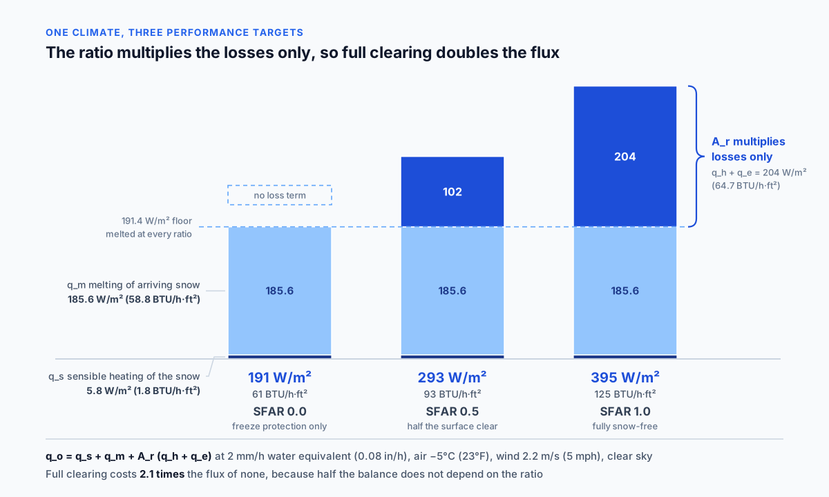
The performance target enters the balance as a multiplier on the loss terms alone. That structural detail explains both why raising the target is expensive and why lowering it to zero fails to make the load disappear.

What the ratio means as a specification:

A_r = 1.0  the whole surface stays visibly clear through the design snowfall
A_r = 0.5  half the surface stays clear, accumulation is accepted on the rest
A_r = 0.0  no snow-free requirement; the duty reduces to freeze protection

Why the multiplier sits where it does:

Snow that lands on the surface has to be melted at any ratio, so q_s and
q_m stand outside the multiplier.

Losses occur only where the warm wet surface is open to the air. Beneath
accumulated snow the surface is insulated and the exchange with the
surroundings very nearly stops.

The three levels evaluated on the one climate used above:

q_s + q_m = 191.4 W/m², losses = 204 W/m²

A_r = 0.0:  191.4 + 0.0 × 204 = 191 W/m² (61 BTU/h·ft²)
A_r = 0.5:  191.4 + 0.5 × 204 = 293 W/m² (93 BTU/h·ft²)
A_r = 1.0:  191.4 + 1.0 × 204 = 395 W/m² (125 BTU/h·ft²)

What follows from the arithmetic:

Going from no snow-free target to a fully clear surface roughly doubles
the required flux and stops there, because half the balance does not
depend on the ratio at all.
The reverse holds as well: even at A_r = 0 the system has to deliver
nearly 200 W/m² (61 BTU/h·ft²), since the snow still has to be melted.
An expectation that relaxing the service level will cut the load several
times over is not borne out.

Who specifies which level:

Full clearing: hospital entrances, emergency vehicle routes, stairs at
  public buildings, airport pavement.
Half: residential driveways and secondary pedestrian routes.
Zero: freeze protection where accumulation is acceptable and the concern
  is ice on a surface that would otherwise be wet.

Per ASHRAE Chapter 52 and PPI Recommendation J: the snow-free area ratio multiplies the loss terms only, since the arriving snow must be melted regardless of the performance target, which is why the load at a zero ratio remains substantial.

Typical Flux Ranges and Why the Two Unit Systems Round Differently

The flux ranges quoted in practice are rules of thumb rounded separately in each unit system, so the metric and Imperial figures printed alongside one another are not exact conversions of each other.

Moderate climates, ordinary applications:  150 to 300 W/m²
Cold climates or a high service level:     300 to 500 W/m² and above
Airport pavement per FAA guidance:         125 to 250 BTU/h·ft²,
                                           which is 394 to 789 W/m²

On the rounding:

The 150 to 300 W/m² range is commonly printed as 50 to 100 BTU/h·ft².
The exact conversion is 47.6 to 95.1, so the Imperial labels are rounded
up by about 5%.
That is acceptable for orientation figures, and it does mean two labels
printed side by side should not be read as a conversion of one another.
The exact factor is 1 BTU/h·ft² = 3.15459 W/m².

Where the order of magnitude comes from:

The balance evaluated above gave 191, 293, and 395 W/m² (61, 93, and
125 BTU/h·ft²) for the three service levels at moderate snowfall and
light wind. Those land inside the published ranges, which is the
evidence that the ranges came out of the same balance.

Why a single universal flux is not available:

The value depends on four independent weather parameters and on a choice
of service level. Borrowing somebody else's number imports their climate
and their client's expectations along with it.

Per ASHRAE Chapter 52, PPI Recommendation J, and FAA Advisory Circular 150/5370-17: published flux ranges are orientation figures derived from the same balance, rounded independently in each unit system, and the design value belongs to a specific city and performance target.

The Load Bands and What They Screen

The calculator classifies the total against four bands.

Metric	Imperial	Category
Below 20 kW	Below 68,250 BTU/h	LOW
20 to 74.9 kW	68,250 to 255,937 BTU/h	MODERATE
75 to 199.9 kW	255,938 to 682,499 BTU/h	HIGH
200 kW and above	682,500 BTU/h and above	VERY HIGH

Consistency between the two systems:

The thresholds were converted exactly. At 3,412.14 BTU/h per kW, 20 kW is
68,243 against a published 68,250, a discrepancy of 0.01%. The other two
edges match to the same precision.
Switching units never changes the category at any input value, which
distinguishes these bands from some others on the site.

What the categories are saying:

LOW: a small walk or driveway, or a conservatively chosen flux.
MODERATE: a typical heated driveway, ramp, or entrance apron.
HIGH: attention needed on heat source, distribution, and zoning.
VERY HIGH: a large system, and a prompt to re-check the area, the flux,
  and the service level before going further.

What they are not saying:

These are size markers, not a verdict on correctness. VERY HIGH on a large
area in a severe climate is entirely normal, and LOW on an understated flux
means only that the assumption was understated.

Per the calculator's stated basis: the bands are illustrative preliminary interpretation ranges rather than code requirements, and they classify size rather than correctness.

Bridge Decks and Elevated Slabs Lose Heat Downward as Well

A slab on grade loses heat downward into soil that eventually warms and slows the loss. An elevated deck loses it to moving air on both faces, which raises the required flux substantially.

The difference in construction:

Slab on grade: soil below, warming through the operating period, usually
  with insulation under the slab. Downward loss is bounded and decays.
Bridge or elevated ramp: open air below at the same temperature as above,
  frequently with wind across it. Downward loss is comparable to the
  upward loss and does not decay.

The order of magnitude:

The underside of an uninsulated elevated deck, at the same temperature
difference and similar exposure, adds a term comparable to the convective
loss from the top face.
Design practice therefore uses a distinctly higher flux for bridges than
for a slab on grade in the same climate. Insulating the underside reduces
the addition without eliminating it.

The same mechanism explains a familiar road hazard: a bridge deck is cooled from both faces and reaches freezing before the adjacent road resting on soil does. A heated bridge deck is fighting precisely that property.

In terms of the calculation:

The calculator has no knowledge of the distinction and accepts the entered
flux as given. For an elevated structure the flux has to come from a source
that accounts for downward loss, or an explicit term has to be added to the
balance.

Per ASHRAE Chapter 52 and FAA Advisory Circular 150/5370-17: elevated slabs lose heat from the underside as well as the surface, requiring a higher design flux than an equivalent slab on grade.

Slab Thermal Inertia and the Hours Before Anything Melts

The load calculation is a steady-state statement. A cold slab has to be warmed to the melting point before any of that steady-state capacity reaches the snow, which takes hours and is the most common reason a correctly sized system appears to fail.

Energy required to warm the slab:

150 mm (6 in) concrete, density 2,400 kg/m³ (150 lb/ft³),
specific heat 880 J/(kg·K) (0.21 BTU/lb·°F),
warmed from −5 to +1°C, a rise of 6 K (10.8°F):

E = 0.15 × 2,400 × 880 × 6 = 1.90 MJ/m² (167 BTU/ft²)

Time at design output:

At 315 W/m² (100 BTU/h·ft²): 1.90e6 / 315 = 6,032 s = 1.7 hours
At 200 W/m² (63 BTU/h·ft²):  1.90e6 / 200 = 9,504 s = 2.6 hours

And that assumes every watt goes into the slab, while some of it leaves
downward and sideways from the start.

What that means during a storm:

A system switched on when the snow starts melts nothing for the first
hours. It is heating the slab.
By the time it reaches operating temperature there is already an
accumulation on the surface, and the system spends the next period
catching up rather than keeping pace.

How the delay is handled:

Idling: the slab is held near freezing through the winter, which removes
  the warm-up entirely and spends energy continuously rather than by event.
Forecast pre-start: the system runs for some hours ahead of expected
  snowfall, which needs a dependable forecast and a controller able to act
  on it.
Snow and moisture sensors in the surface: the system starts on the first
  precipitation, and accepts the warm-up delay that follows.

Why inertia stays out of the load calculation:

The design flux is a steady-state quantity. Inertia determines when that
quantity begins doing the job it was sized for, which is a control question
rather than a capacity question.

Per ASHRAE Chapter 52 and PPI Recommendation J: the steady-state flux calculation does not include the energy required to bring a cold slab to the melting point, which for typical construction takes on the order of two hours at design output.

Idling and Why Installed Capacity Is Not Annual Energy

The calculator sizes equipment for the design storm. Operating cost is set by how the system is run between storms, and the two questions have almost nothing to do with one another.

Two separate quantities:

Installed capacity: set by the design storm and the service level. This is
  what the calculator produces.
Annual energy: set by run hours, idling strategy, and controls. The
  calculator says nothing about it.

What idling does to the second one:

Holding the slab near freezing all winter removes the warm-up delay and
converts the system from event-driven to continuous.
Run hours rise by an order of magnitude even though the idling output is
a fraction of the design output.

Controls as the main lever:

Precipitation and surface moisture sensors start the system only when
there is snow, rather than on temperature alone.
Temperature-only control runs the system through every cold dry night,
when there is nothing on the surface to melt.
Energy standards require automatic control for this reason.

Zoning:

Splitting a large area into zones allows priority sections to be held
fully clear while secondary sections run at a lower service level, which
reduces both peak source capacity and consumption.

Per ASHRAE Standard 90.1-2022 and ASHRAE Chapter 52: snow melt systems require automatic controls responding to moisture and temperature together, because temperature-only control runs the system through every cold dry night, and operating energy is governed by run hours rather than by installed capacity.

Worked Example: 120 Square Metres at 300 Watts per Square Metre

The metric example on the calculator page, followed through to what the flux implies.

Heated area:      120 m² (1,292 ft²)
Design heat flux: 300 W/m² (95.1 BTU/h·ft²)

Step 1. Total load.

Total = 120 × 300 = 36,000 W = 36 kW (122,837 BTU/h)

Step 2. Ton equivalent.

36,000 / 3,517 = 10.24 tons
Quoted for comparison only; this is a heating system.

Step 3. Category.

36 kW falls in the 20 to 74.9 kW band → MODERATE
122,837 BTU/h falls in 68,250 to 255,937 BTU/h → MODERATE
The two systems agree.

Step 4. What service level that flux corresponds to.

From the balance evaluated earlier, at 2 mm/h water equivalent, air −5°C
(23°F), and wind 2.2 m/s (5 mph):
  A_r = 0.0 → 191 W/m² (61 BTU/h·ft²)
  A_r = 0.5 → 293 W/m² (93 BTU/h·ft²)
  A_r = 1.0 → 395 W/m² (125 BTU/h·ft²)
The entered 300 W/m² corresponds to roughly half the surface staying
clear in that climate.

Step 5. What full clearing would cost.

At A_r = 1.0 the flux is 395 W/m², so 120 × 395 = 47.4 kW
(161,735 BTU/h), a rise of 32% over 36 kW.
The category stays MODERATE, but the heat source and the loop are
designed to the larger figure.

Step 6. The same target on an exposed site.

At a design wind of 6.7 m/s (15 mph) the losses rise to about 350 W/m²
and the full-clearing flux reaches 540 W/m² (171 BTU/h·ft²).
The load becomes 120 × 540 = 64.8 kW (221,107 BTU/h), 1.8 times the
original, at the same snowfall and the same air temperature.

Step 7. Time to reach operating temperature.

150 mm (6 in) slab warmed 6 K (10.8°F): 1.90 MJ/m² (167 BTU/ft²).
At 300 W/m² that is 6,336 s, about 1.8 hours before melting starts,
if the system begins from a cold slab.

Step 8. What to specify at the source.

36 kW (122,837 BTU/h) at design conditions, plus margin for warm-up if
rapid start is expected rather than idling.
The loop is outdoors, so it runs on glycol, which lowers the specific
heat of the fluid and raises the flow rate needed for the same duty.

Step 9. The glycol correction.

A 30% solution lowers specific heat from about 4.19 to about 3.7
kJ/(kg·K), close to 12%, so the flow rate rises by a corresponding
amount at the same temperature difference and the same transferred power.

Step 10. The result.

36 kW (122,837 BTU/h), 10.24 tons, MODERATE.
The 300 W/m² flux corresponds to roughly half clearing at moderate
snowfall and light wind. Full clearing would need 47.4 kW, and full
clearing on an exposed site 64.8 kW.

That figure then feeds heat source selection, loop design, and the choice of glycol concentration.

Imperial Worked Example and the Flux It Implies

The Imperial example on the calculator page, and what it says about the width of the bands.

Heated area:      1,000 ft² (92.9 m²)
Design heat flux: 100 BTU/h·ft² (315.5 W/m²)

Total = 1,000 × 100 = 100,000 BTU/h (29.3 kW)
Tons  = 100,000 / 12,000 = 8.33
Category: 68,250 to 255,937 BTU/h → MODERATE

Cross-check in the other system:

29.3 kW falls in the 20 to 74.9 kW band → MODERATE
The categories agree, as they should when the thresholds convert exactly.

What service level this flux implies:

315.5 W/m² sits between the values for A_r = 0.5 (293 W/m²) and A_r = 1.0
(395 W/m²), nearer to half clearing, in the same moderate climate.

The two page examples set against each other:

Metric:   120 m² at 300 W/m²   → 36 kW
Imperial: 92.9 m² at 315.5 W/m² → 29.3 kW
The area is 23% smaller, the flux is 5% higher, the total is 19% lower.
Both land in the same category, which says something about band width:
MODERATE spans nearly a fourfold range of load.

Sensitivity to the two inputs:

The load is linear in each field, so an error in either passes into the
result one for one.
The area is usually known accurately. The flux is not, and essentially
all of the uncertainty in the answer lives in the second field.

What a wide band means when reading a result:

MODERATE covers 20 to 74.9 kW (68,250 to 255,937 BTU/h). Two projects
inside it can differ several times over in the cost of the heat source
and the loop, so the band indicates scale rather than substituting for
the calculation.

Per the calculator's model: the load is linear in both inputs, so the uncertainty of the result is the uncertainty of the design flux, and the interpretation bands are wide enough that a single category covers a large range of practical system sizes.

Application Boundaries: Weather Basis, Transients, Detailed Design

The calculator covers the product of area and a stated flux, and the assignment of that product to a size band. The following require separate treatment.

Selection of the design flux. The calculator does not determine it. The value comes from ASHRAE climate data for the specific city together with the chosen snow-free area ratio.

Frequency basis. ASHRAE design proceeds from the fraction of snowfall hours the system is expected to handle rather than from a single worst hour. Choosing that fraction is a design decision with cost attached.

Transient behaviour. The model is steady-state. Slab warm-up, the response at the onset of snowfall, and behaviour through breaks in precipitation are not represented.

Thermal inertia. The energy needed to bring a cold slab to the melting point is outside the calculation and amounts to roughly two hours of operation at design output.

Bridges and elevated structures. Downward loss is not included, and for elevated construction it is significant.

Loop design. Tube spacing, fluid temperature, flow rate, zoning, control scheme, and heat source selection all sit beyond this calculation.

Electric heating. For cable systems the resulting power converts into cable wattage density, circuit count, and protection parameters, which fall under electrical codes rather than under this model.

Glycol. An outdoor loop runs on antifreeze, which lowers specific heat and raises viscosity, changing both the required flow rate and the pump curve it has to be selected against.

Annual energy. Governed by run hours and control strategy rather than by installed capacity.

Per ASHRAE Handbook, HVAC Applications (2023), Chapter 52 and PPI Recommendation J: the area times flux product is a preliminary sizing step, while flux selection from city climate data, frequency basis, transient behaviour, elevated-slab losses, loop design, and control strategy require separate treatment.

Snow Melt System Sizing Calculator

Standards and References

• ASHRAE Handbook, HVAC Applications (2023), Chapter 52, Snow Melting and Freeze Protection. The surface energy balance, the snow-free area ratio, city-by-city climate data, and the frequency basis for selecting a design flux.
• ASHRAE Handbook, Fundamentals (2025), Chapter 4, Heat Transfer. Convective and radiative exchange between a surface and its surroundings, evaporation from a wetted surface, and the Stefan-Boltzmann constant in both unit systems.
• PPI Recommendation J, Hydronic Snow and Ice Melting Systems. Application of Chapter 52, selection of service level, loop construction and tube spacing, and slab thermal inertia.
• FAA Advisory Circular 150/5370-17, Airside Use of Heated Pavement Systems. Design fluxes for airfield pavement, worked calculation examples, and the treatment of elevated structures.
• ASHRAE Standard 90.1-2022, Energy Standard for Buildings Except Low-Rise Residential Buildings. Automatic control requirements applicable to outdoor surface heating systems.
• NFPA 70, National Electrical Code (2023), articles covering fixed outdoor de-icing and snow-melting equipment. Circuit, protection, and installation requirements for electric systems.
• IEEE Std 515-2017, Testing, Design, Installation and Maintenance of Electrical Resistance Trace Heating for Industrial Applications. Design requirements for resistance heating cable systems.
• Manufacturer data for hydronic tubing and heating cable (2020 onward). Tube spacing, cable wattage density, permissible fluid temperature, and burial depth.
• Literature on concrete slab thermal inertia and the response time of outdoor heating systems, including control guidance for precipitation and surface moisture sensing.

FAQ

Related Calculators

• Glycol Concentration Calculator: The antifreeze concentration in the outdoor loop, which lowers specific heat and raises the flow rate needed for the same duty (article).
• Hydronic Balancing Calculator: Flow distribution between the loops embedded in the heated slab, which decides whether the surface clears evenly (article).
• Boiler Efficiency Calculator: The heat source that has to cover the calculated capacity through the design storm, where the fuel input behind 36 kW of surface output depends on the efficiency at the low return temperature a slab loop returns.
• Heat Exchanger Calculator: The separation between the boiler primary circuit and the outdoor glycol loop (article).
• District Heating Pipe Loss Calculator: Losses in the buried mains carrying heat out to the melted area, which add to what the source has to produce (article).
• Boiler Feed Pump Sizing: Pump selection against the flow rate that the glycol correction has already raised by roughly a tenth.
• Pool Heating Load: The adjacent case of heating an open surface outdoors, where evaporation carries a large share of the loss and wind moves the answer the same way it does here.
• Ground Source Heat Pump COP Estimator: An alternative source for systems built around a low loop temperature, which suits a slab better than it suits a radiator circuit.