District Heating Pipe Heat Loss: The Cylindrical Resistance Model, Linear Loss in Watts per Metre, and Annual Energy Cost

Why a District Heating Network Loses Heat Every Metre of the Way

A district heating network pays a continuous thermal tax: every metre of buried pipe between the plant and the customer leaks heat into the ground around the clock, and because the network runs year after year at 8,760 hours, a loss rate that sounds trivial per metre becomes a large annual energy and cost figure. A 10 W/m loss on a 50-kilometre network accumulates to 4,380 MWh per year, the equivalent of several hundred tonnes of fuel.

Hot water leaves the plant at supply temperature and travels through pre-insulated buried pipe toward the buildings it serves. Heat conducts radially outward through the carrier pipe wall, then through the polyurethane foam insulation, into the surrounding soil. The rate is set by the temperature difference divided by the thermal resistance of the layers. A well-insulated pipe might lose 20 watts per metre, which sounds small until multiplied by network length and annual hours: a kilometre of pipe at 30 W/m loses roughly 260 megawatt-hours a year, about the annual heating demand of fifteen homes.

The calculator applies the cylindrical multi-layer resistance model to compute linear heat loss in watts per metre or BTU per hour per foot, then extends it to total loss, annual energy, cost, insulation efficiency, and, when flow is given, the return temperature. It continues the hydronic sub-cluster after the fluid (glycol) and the flow distribution (balancing), addressing what the distribution itself costs. The same buried geometry appeared in the Buried Pipe Heat Loss article with a soil conduction shape factor; this district heating model treats the ground temperature as a boundary at the insulation surface, an assumption Section 8 examines. EN 15698 defines the thermal performance classes the result is judged against.

Calculator Inputs: Geometry, Temperatures, Materials, and the Optional Economics

The calculator collects twelve inputs and extends the result to energy and cost when optional fields are populated.

Unit System. Imperial (inches, °F, feet, BTU/h·ft, GPM, $/MMBTU) or Metric (mm, °C, m, W/m, L/min, $/kWh). The choice sets every labeled unit on the page.

Pipe Inner Diameter [in or mm]. Inside diameter of the carrier pipe, from which the inner radius r_pi is derived. Typical district heating DN 100 carrier: 100 mm (4 in).

Pipe Outer Diameter [in or mm]. Outside diameter of the carrier pipe, giving r_po. Both inner and outer are needed because the wall carries its own resistance (small for carbon steel, larger for stainless), and the outer diameter sets where the insulation begins.

Insulation Thickness [in or mm]. Radial thickness of the foam layer. The insulation outer radius is r_ins = r_po + thickness. A 50 mm (2 in) polyurethane jacket is typical for a Series 1 pre-insulated pipe on a DN 100 carrier.

Supply Water Temperature [°F or °C]. Hot water temperature at the start of the section. Conventional district heating runs 70–120°C (158–248°F); fourth-generation low-temperature networks run lower.

Ground Temperature [°F or °C]. Average soil temperature at burial depth. An annual average suits a full-year energy estimate; in temperate climates this is typically 8–12°C (46–54°F).

Pipe Length [ft or m]. One-way length of the buried section, not round-trip. Entering round-trip distance doubles the reported loss for that pipe.

Pipe Thermal Conductivity. Carbon steel: 50 W/m·K (29 BTU/h·ft·°F). Stainless steel 316: 16 W/m·K (9.2 BTU/h·ft·°F). Copper: 386 W/m·K (223 BTU/h·ft·°F).

Insulation Thermal Conductivity. Polyurethane foam: 0.027 W/m·K (0.0156 BTU/h·ft·°F). Mineral wool: 0.035 W/m·K (0.0202 BTU/h·ft·°F). Fiberglass: 0.040 W/m·K (0.0231 BTU/h·ft·°F). Aerogel: 0.023 W/m·K (0.0133 BTU/h·ft·°F).

Flow Rate [GPM or L/min, optional]. When entered, enables the return temperature and temperature drop per unit length output.

Energy Price [$/MMBTU or $/kWh, optional]. Enables the annual cost calculation.

Operating Hours per Year [optional, default 8,760]. Annual run hours for the energy and cost calculation.

Calculator outputs: Linear Heat Loss Rate (W/m or BTU/h·ft), Total Heat Loss (W or BTU/h), Annual Heat Loss (kWh/yr or MMBTU/yr), Annual Energy Cost ($/yr when price is entered), Return Temperature (°F or °C when flow is entered), Temperature Drop per Unit Length, and Insulation Efficiency (%).

The calculator does not account for soil thermal resistance as a separate input (ground temperature is a fixed boundary), surface convection at the outer jacket surface (buried assumption), thermal bridges at joints and fittings, the supply-and-return pair together (single pipe only), seasonal ground-temperature variation, adjacent-pipe interaction, or network branching.

Multi-Layer Cylindrical Resistance: Why Each Layer Is a Logarithm

Each concentric layer of a buried pipe contributes a thermal resistance proportional to the logarithm of its radius ratio, because heat spreading radially outward passes through a surface area that grows with radius.

R_pipe = ln(r_po / r_pi) / (2π × λ_pipe)     [K·m/W or h·ft·°F/BTU]
R_ins  = ln(r_ins / r_po) / (2π × λ_ins)
R_total = R_pipe + R_ins

where:
  r_pi  = carrier pipe inner radius [m or ft]
  r_po  = carrier pipe outer radius [m or ft]
  r_ins = insulation outer radius = r_po + thickness [m or ft]
  λ     = thermal conductivity of the layer [W/m·K or BTU/h·ft·°F]

Linear heat loss:

q = (T_supply − T_ground) / R_total     [W/m or BTU/h·ft]

In a flat wall, resistance equals thickness divided by (k × area), because the area is constant. In a cylinder, the area grows with radius (A = 2πrL), so each successive shell of material has more area to conduct through and adds less resistance than the last. Integrating the heat equation in cylindrical coordinates gives ln(r_outer/r_inner)/(2πk), the logarithmic form codified in ISO 12241:2008 and ASHRAE Fundamentals.

The logarithm has two important consequences. Doubling insulation thickness does not halve the loss: each added layer sits at a larger radius, with more surface area, contributing less resistance per unit added. Insulation shows diminishing returns with thickness:

Doubling thickness roughly halves loss at small radius ratios.
Adding 25 mm to an existing 50 mm layer cuts loss by about 40%.
Each further increment contributes less than the last.

The formula uses radii. Entering diameters gives the same ratio (d_o/d_i = r_o/r_i), which is correct; mixing a diameter with a radius corrupts the result. Layers in series add directly: R_total = R_pipe + R_ins.

Worked metric example:

r_pi = 0.050 m, r_po = 0.057 m, r_ins = 0.107 m
R_pipe = ln(0.057/0.050) / (2π × 50) = 0.1310/314.16 = 0.000417 K·m/W
R_ins  = ln(0.107/0.057) / (2π × 0.027) = 0.6296/0.1696 = 3.712 K·m/W
R_total = 3.712 K·m/W

Per ISO 12241:2008 and ASHRAE Fundamentals: each concentric layer contributes ln(r_outer/r_inner)/(2πλ), because conducting area grows with radius. Layers add in series; linear loss is the temperature difference divided by the total. The logarithm is why insulation thickness shows diminishing returns with each additional layer.

Insulation Dominance: The Pipe Wall Contributes Almost Nothing

In a pre-insulated district heating pipe the insulation carries essentially all the thermal resistance, and the steel carrier wall contributes so little that it is nearly invisible in the total.

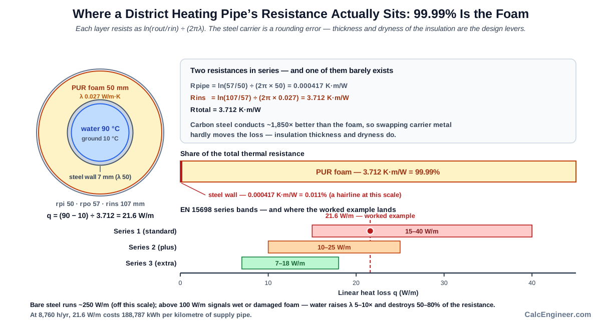
The magnitude gap comes directly from the conductivity ratio:

Carbon steel λ ≈ 50 W/m·K (29 BTU/h·ft·°F)
Polyurethane foam λ ≈ 0.027 W/m·K (0.0156 BTU/h·ft·°F)
Steel conducts roughly 1,850 times better than the foam.

Worked comparison, metric:

R_pipe = 0.000417 K·m/W
R_ins  = 3.712 K·m/W
The wall is 0.011% of the total; the insulation carries 99.99%.

Imperial equivalent:

R_pipe = 0.000647 h·ft·°F/BTU,  R_ins = 6.49 h·ft·°F/BTU
The wall is 0.01% of the 6.49 total.

Both pipe diameters are still required as inputs. The model needs the exact geometry, and while the wall resistance is negligible for carbon steel, it is three times larger for stainless steel (λ ≈ 16 W/m·K), which matters for specialty carrier materials. The outer diameter also sets where the insulation begins, so the inner diameter alone does not define the geometry.

The design consequence is direct: changing the carrier pipe material barely moves the linear loss. Changing insulation thickness or conductivity moves it substantially. Above-ground pipe differs because an outer air-film convection resistance joins the series; buried pipe omits that resistance, and Section 8 explains why.

Per EN 15698-2:2019 and manufacturer data (Logstor, Isoplus, Perma-Pipe): insulation carries 99.9% or more of a pre-insulated pipe's thermal resistance, since steel conducts roughly 1,850 times better than polyurethane foam. Design attention belongs on insulation thickness and conductivity, not the carrier metal.

Linear Heat Loss: The Metric District Heating Is Judged On

District heating performance is expressed as linear heat loss, watts per metre or BTU per hour per foot, because it normalizes the loss against network length and lets pipes of any size and length be compared on a single number.

q = (T_supply − T_ground) / R_total   [W/m or BTU/h·ft]
Q = q × L                             [W or BTU/h, total for the section]

Total loss depends on how long the network is, which makes it uninformative across projects of different scale. Linear loss isolates the pipe's thermal quality, comparable between a 200 m branch and a 20 km transmission main. A pipe that achieves 15 W/m performs the same whether it is 100 m or 10,000 m long; only the total energy consequence scales with length.

Typical ranges for pre-insulated pipe:

Well-insulated pre-insulated pipe:  7–45 W/m (7–47 BTU/h·ft), depending on size and temperature
Bare steel pipe (DN 100, 90°C):     ~250 W/m (260 BTU/h·ft), 10–20× a good insulated pipe
Above 100 W/m (104 BTU/h·ft):      critical threshold, indicating damage or missing insulation

What drives it: temperature difference (supply minus ground) is directly proportional; insulation thickness acts logarithmically with diminishing returns; insulation conductivity is inversely proportional (wet insulation is devastating, as Section 10 addresses); pipe diameter has an indirect effect because a larger carrier surface means more loss for the same insulation thickness.

Multiply linear loss by length to get the section total, then by annual hours to get energy. Small differences in W/m become large annual figures at network scale. A district heating circuit has both a supply pipe and a return pipe, each losing heat. This calculator models one pipe; a full circuit needs both run separately. The return pipe loses less, being cooler, but the loss is not zero. Section 14 covers this scope boundary.

Per EN 15698:2019 and Euroheat & Power benchmarks: linear heat loss (W/m or BTU/h·ft) is the district heating performance metric, normalizing loss against length. Well-insulated pipe runs 7–45 W/m; bare steel around 250 W/m; above 100 W/m signals a problem.

EN 15698 Series Classes and the Loss Ranges They Define

European practice classifies pre-insulated pipe by insulation series, and the series a project specifies sets both its linear loss and its long-term economics.

The series definitions from EN 15698-1:2019:

Series	Insulation	Typical linear loss
Series 1	Standard thickness	15–40 W/m (16–42 BTU/h·ft)
Series 2	Plus (thicker)	10–25 W/m (10–26 BTU/h·ft)
Series 3	Extra (thickest)	7–18 W/m (7–19 BTU/h·ft)

Higher series means thicker insulation at the same carrier size, a lower linear loss, and a larger outer jacket diameter. Series 2 and 3 cost more in material and trench width, and save energy every hour of operation. The additional cost of thicker insulation is typically recovered within 3–7 years through energy savings. Beyond that, the saving is ongoing for the pipe's service life, measured in decades.

The logarithm governs the economics. Going from Series 1 to Series 2 saves substantially: a step from roughly 30 W/m to 18 W/m, about a 40% reduction. Going from Series 2 to Series 3 saves less, because each added shell of foam sits at a larger radius and contributes less resistance:

Doubling thickness roughly halves loss at first.
Adding 25 mm to an existing 50 mm layer cuts loss by about 40%.
Further additions give smaller improvements.

Buried pipe stays in the ground for decades. Re-insulating means excavation, which is expensive and disruptive. The insulation decision is effectively permanent, which favors the higher series where the network runs continuously.

EN 15698-1:2019 covers requirements for pre-insulated bonded systems, where the carrier pipe, foam insulation, and outer jacket are bonded together into a factory-assembled unit. EN 15698-2:2019 covers the thermal calculation and design of buried systems. EN 253:2019 covers bonded single-pipe systems used in the majority of installations.

Per EN 15698-1:2019 and EN 15698-2:2019: pre-insulated pipe is classified in Series 1 (15–40 W/m), Series 2 (10–25 W/m), and Series 3 (7–18 W/m). Thicker series typically pay back in 3–7 years. The logarithmic relation means each step up saves less than the last.

The Ground as a Fixed Boundary: What This Model Assumes About Soil

This model treats the ground temperature as a fixed boundary at the outside of the insulation, adding no soil resistance and no surface convection, which is a deliberate simplification whose direction and magnitude are worth understanding.

What the model includes and omits:

Included:  R_pipe (carrier wall) + R_ins (insulation)
Omitted:   R_soil (conduction spreading through the ground to the surface)
Omitted:   outer surface convection (a buried pipe has no air film)

Omitting surface convection is correct. A buried pipe is in direct contact with soil, not air, so there is no surface air film to include. The buried case legitimately has no convection resistance at the outer jacket surface; this omission is appropriate, not a simplification.

Omitting soil resistance is conservative: real soil adds resistance between the insulation surface and the ground above. The calculated loss is therefore higher than reality, which is safe for design. The magnitude of this correction: soil resistance is typically a few tenths of a K·m/W, against an insulation resistance of several K·m/W. For a well-insulated pipe the correction is modest. For a poorly insulated or bare pipe, soil resistance becomes dominant, and this model overstates loss substantially.

The alternative for bare or lightly insulated pipe uses the soil shape-factor:

R_soil = acosh(2z/D) / (2π × k_soil)

z      = burial depth to pipe centre [m or ft]
D      = buried outer diameter [m or ft]
k_soil = soil thermal conductivity [W/m·K or BTU/h·ft·°F]

That approach suits bare or lightly insulated buried pipe and soil-sensitivity studies. The district heating model suits pre-insulated pipe where insulation dominates and the conservative ground-boundary assumption is a small correction. The Buried Pipe Heat Loss article covers the soil shape-factor treatment; the two articles form a cross-cluster pair with distinct modeling assumptions for the same buried geometry.

The ground temperature entered should be the temperature at burial depth, not the air temperature. Annual average soil temperature at typical district heating burial depth (0.8–1.5 m) is appropriate for a full-year energy estimate.

Per EN 15698-2:2019 and ISO 12241:2008: this model uses pipe and insulation resistance with ground temperature as a fixed boundary, omitting soil conduction and surface convection. The omission is conservative (loss overstated) and small for well-insulated pipe. Bare or degraded pipe, or soil-sensitivity work, calls for a soil shape-factor treatment instead.

Insulation Efficiency and How to Read a Number Near One Hundred

The calculator reports an insulation efficiency comparing the insulated pipe against a bare one, and because the bare reference in this model has only the steel wall to resist heat flow, the figure sits very close to 100% and should be read as a relative indicator rather than an absolute score.

The definition:

η_ins = (1 − q / q_bare) × 100%
q_bare = (T_supply − T_ground) / R_pipe     (pipe-wall resistance only)

For carbon steel at the worked example geometry, R_pipe is approximately 0.000647 h·ft·°F/BTU, essentially zero resistance. So q_bare is enormous: in the Imperial example, 200,927 BTU/h·ft. Against that reference, an insulated pipe at 20.0 BTU/h·ft scores 99.99%. The metric equivalent gives the same result: 0.000417 K·m/W wall against 3.712 K·m/W total.

How to read it: treat the efficiency figure as a relative indicator across cases, not an absolute performance score. A drop from 99.99% to 99.9% represents a tenfold increase in loss, which is significant. The primary number to judge performance on is the linear loss in W/m compared to the EN 15698 series ranges (Section 7).

A lower figure signals trouble: efficiency falling below about 80% in this framing indicates insulation that is degraded, wet, or missing, and warrants investigation. Compare the calculated linear loss against the EN 15698 series ranges, or against measured supply-return temperatures on the section; that comparison is more informative than a percentage pinned near 100.

Note on the physical reference: a physically bare buried steel pipe would be limited by soil resistance, not by the steel wall, losing on the order of 250 W/m rather than the model's arithmetic reference. The efficiency figure uses the model's internal reference, not that physical case.

Per EN 15698 practice and the calculator's definition: insulation efficiency compares loss against a pipe-wall-only reference, so the value sits near 100%. Read it relatively; judge performance on linear loss in W/m against the series ranges. Below roughly 80% indicates degraded, wet, or missing insulation.

Wet Insulation: The Five-to-Ten-Times Conductivity Failure

The most common cause of excessive district heating loss is not thin insulation but wet insulation, because water intrusion multiplies the foam's thermal conductivity several-fold and destroys most of its resistance.

Polyurethane foam insulates because its closed cells trap gas, which is a poor conductor. Water entering the foam replaces that gas with a far better conductor. Conductivity can rise 5 to 10 times; thermal resistance falls correspondingly. Wet insulation can lose 50–80% of its thermal resistance. A pipe designed at 20 W/m can climb well past 100 W/m, the critical threshold.

Water gets in through jacket damage during installation or backfill compaction, joint or field-weld casing failures, ground-water ingress at fittings and branches, and age-related jacket degradation. Pre-insulated bonded systems are designed to prevent this, but any breach in the outer jacket opens a path for moisture.

Detection: compare measured supply and return temperatures against values calculated for the section. Sections whose measured loss exceeds the calculation by a significant margin likely have wet or damaged insulation. Pre-insulated systems often include alarm wires embedded in the foam that change resistance when wetted, providing an early warning before the thermal penalty becomes large.

Modeling a wet section in the calculator: raise the insulation conductivity input to reflect the wet condition (5–10 times the dry value) and compare the resulting linear loss against the measured behavior. This brackets the expected loss range and supports the case for section replacement.

Replacing a wet section is high-return: the loss reduction is large and immediate, unlike marginal thickness upgrades on healthy pipe. Per EN 15698 practice and manufacturer guidance (Logstor, Isoplus, Perma-Pipe): water intrusion raises foam conductivity 5–10 times and can destroy 50–80% of thermal resistance, pushing a well-designed pipe past the critical loss threshold.

Return Temperature and the Low-Temperature Network Case

When flow is entered, the model also reports the return temperature, and that number matters beyond the pipe itself, because a low return temperature is what allows a district heating plant to run condensing boilers, integrate heat pumps, and absorb recovered heat at higher efficiency.

The relation:

T_return = T_supply − Q / (ṁ × cp)

ṁ  = mass flow rate [lb/h or kg/s]
cp = 1.0 BTU/lb·°F (4,190 J/kg·K) for water
Q  = total heat loss over the section [BTU/h or W]

Imperial mass flow from GPM:

ṁ = flow [GPM] × 8.33 lb/gal × 60 min/h   [lb/h]
200 GPM → 200 × 8.33 × 60 = 99,960 lb/h

For the worked example (20,000 BTU/h over 1,000 ft at 200 GPM):

ΔT = 20,000 / (99,960 × 1.0) = 0.20°F
T_return = 180 − 0.20 = 179.8°F (82.1°C)

The temperature drop from pipe loss is small at high flow over a short section. The large temperature drop in a real network happens at the consumer substations, where heat is deliberately extracted. Pipe heat loss is the background loss between substations.

Flow rate does not change linear loss. The watts per metre leaving the pipe depend on temperatures and thermal resistances, not on flow. Higher flow reduces the temperature drop along the pipe because more thermal mass carries the same lost heat, but the pipe still emits the same watts per metre outward.

Below 40°C (104°F), a plant can run condensing boilers, recovering latent heat from flue gas, integrate heat pumps at higher COP, and use solar thermal or waste heat sources. Low-temperature, fourth-generation district heating is built around this principle. High return temperature signals poor extraction at consumer substations or excessive network distribution loss upstream.

Per ASHRAE Handbook HVAC Systems and Equipment (District Heating and Cooling) and fourth-generation district heating literature: return temperature follows from the heat removed and the mass flow. Flow rate does not change linear loss, only the temperature drop. Return below 40°C (104°F) enables condensing boilers, heat pumps, and recovered heat.

Worked Example: A 4-Inch Carrier at 20 BTU per Hour per Foot

Buried pre-insulated district heating branch, carbon steel carrier. Pipe inner diameter 4 in (100 mm nominal), outer diameter 4.5 in (114 mm), insulation 2 in (50 mm) polyurethane foam. Supply 180°F (82.2°C), ground 50°F (10.0°C), length 1,000 ft (305 m). Conductivities: λ_pipe = 29 BTU/h·ft·°F (50 W/m·K), λ_ins = 0.0156 BTU/h·ft·°F (0.027 W/m·K). Flow 200 GPM, 8,760 h/yr, energy $10/MMBTU.

Step 1. Radii in feet:

r_pi = 2.00 in = 0.16667 ft
r_po = 2.25 in = 0.18750 ft
r_ins = 2.25 + 2.00 = 4.25 in = 0.35417 ft

Step 2. Pipe wall resistance:

R_pipe = ln(0.18750/0.16667) / (2π × 29)
       = ln(1.1250) / 182.21
       = 0.11778 / 182.21
       = 0.000647 h·ft·°F/BTU

Step 3. Insulation resistance:

R_ins = ln(0.35417/0.18750) / (2π × 0.0156)
      = ln(1.8889) / 0.09802
      = 0.63611 / 0.09802
      = 6.49 h·ft·°F/BTU

Step 4. Total resistance:

R_total = 0.000647 + 6.49 = 6.49 h·ft·°F/BTU
The wall is 0.01% of the total; insulation governs.

Step 5. Linear heat loss:

q = (180 − 50) / 6.49 = 130 / 6.49 = 20.0 BTU/h·ft (19.2 W/m)

Step 6. Total heat loss:

Q = 20.0 × 1,000 = 20,000 BTU/h (5.86 kW)

Step 7. Annual energy:

E = 20,000 × 8,760 / 1,000,000 = 175.2 MMBTU/year (51,340 kWh/year)

Step 8. Annual cost:

Cost = 175.2 × $10 = $1,752/year for this 1,000 ft supply branch

Step 9. Return temperature at 200 GPM:

ṁ = 200 × 8.33 × 60 = 99,960 lb/h
ΔT = 20,000 / (99,960 × 1.0) = 0.20°F
T_return = 180 − 0.20 = 179.8°F (82.1°C)

Step 10. Insulation efficiency:

q_bare = 130 / 0.000647 = 200,927 BTU/h·ft (pipe-wall reference)
η_ins  = (1 − 20.0/200,927) × 100 = 99.99%

Read the efficiency figure relatively (Section 9); judge performance on the 20.0 BTU/h·ft value.

Result. 20.0 BTU/h·ft (19.2 W/m) is a low linear loss, consistent with EN 15698 Series 2 or better. The annual cost is $1,752 for this 1,000 ft supply branch alone. Scale to full network length and add the return pipe for the circuit total. Cross-reference the Buried Pipe Heat Loss article for the soil shape-factor treatment of the same geometry, and the Hydronic Balancing article for distributing the delivered flow across consumer circuits.

Metric Worked Example and the Annual Energy Economics

Same pipe geometry in metric units. Pipe inner diameter 100 mm (r_pi = 0.050 m), outer 114 mm (r_po = 0.057 m), insulation 50 mm polyurethane (r_ins = 0.107 m). Supply 90°C (194°F), ground 10°C (50°F), length 1,000 m (3,281 ft). λ_pipe = 50 W/m·K, λ_ins = 0.027 W/m·K.

Step 1. Pipe wall resistance:

R_pipe = ln(0.057/0.050) / (2π × 50)
       = ln(1.14) / 314.16
       = 0.1310 / 314.16
       = 0.000417 K·m/W

Step 2. Insulation resistance:

R_ins = ln(0.107/0.057) / (2π × 0.027)
      = ln(1.877) / 0.1696
      = 0.6296 / 0.1696
      = 3.712 K·m/W

Step 3. Total resistance:

R_total = 0.000417 + 3.712 = 3.712 K·m/W
The wall is 0.011% of the total.

Step 4. Linear heat loss:

q = (90 − 10) / 3.712 = 80 / 3.712 = 21.6 W/m (22.4 BTU/h·ft)

Step 5. Total heat loss:

Q = 21.6 × 1,000 = 21,551 W (73,530 BTU/h)

Step 6. Annual energy:

E = 21,551 × 8,760 / 1,000 = 188,787 kWh/year (644 MMBTU/year)

That is 188,787 kWh from a single kilometre of supply pipe. At district heating network scale, tens of kilometres times this per-kilometre figure makes distribution loss a leading efficiency term for the whole network. A network with 50 km of this pipe loses over 9,000 MWh per year on the supply side alone before the return pipe is counted.

Series comparison:

21.6 W/m sits in the LOW to MODERATE range, consistent with EN 15698 Series 1 to 2.
A Series 3 pipe on the same carrier would reach 10–15 W/m.

Upgrade arithmetic:

Cutting loss from 21.6 to 15 W/m saves 6.6 W/m.
Over 1,000 m and 8,760 h: 6.6 × 1,000 × 8,760 / 1,000 = 57,816 kWh/year saved.

That saving continues for the buried life of the pipe, which is why the thicker series typically pays back in 3–7 years on a continuously operating network. Insulation carries 99.99% of the resistance; thickness and dryness are the levers.

Per EN 15698-2:2019 and Euroheat & Power: the metric case gives 21.6 W/m and 188,787 kWh per year per kilometre. Reducing to 15 W/m saves roughly 58,000 kWh a year per kilometre, the arithmetic behind the 3–7 year payback on a higher insulation series.

Application Boundaries: Supply-Return Pairs, Joints, Seasonal Ground, Networks

This calculator's scope is a single buried pre-insulated pipe at steady state, with pipe wall and insulation resistance and ground temperature as a fixed boundary. Several situations require separate treatment.

Supply and Return Together. The model covers one pipe. A district heating circuit has both a supply and a return pipe, each losing heat. The return loses less, being cooler, but the loss is not zero. Total circuit loss requires both pipes analyzed separately and summed.

Adjacent Pipe Interaction. Supply and return pipes in a shared trench warm the soil between them, changing both pipes' losses. Twin-pipe and shared-trench thermal interaction requires a multi-pipe treatment beyond this single-pipe model.

Soil Resistance and Burial Depth. Ground temperature is a fixed boundary; soil conduction and burial depth are not inputs (Section 8). Depth-sensitivity studies and bare-pipe work require a soil shape-factor model, covered in the Buried Pipe Heat Loss article.

Thermal Bridges. Joints, fittings, valves, anchors, and casing penetrations lose more per unit length than the straight pipe. These are not modeled; add per-item allowances or equivalent-length factors from manufacturer data.

Seasonal Ground Temperature. The model uses one ground temperature. Real soil temperature swings seasonally at burial depth; an annual average suits an annual estimate, and seasonal analysis needs the monthly ground temperature profile.

Above-Ground Sections. The model omits surface convection, correct for buried pipe only. Above-ground runs need an added outer film resistance. This model underestimates heat loss for above-ground sections.

Wet or Degraded Insulation. The model uses the entered conductivity without adjustment. Wet foam needs the conductivity raised 5–10 times (Section 10) to reflect the actual condition.

Network Analysis. This is a single-section estimate. Branching networks with varying load profiles, hydraulic interaction, and demand diversity require district heating simulation software.

Length Basis. The model uses one-way length. Entering round-trip distance doubles the reported loss for that pipe.

Per EN 15698-2:2019 and ASHRAE Handbook HVAC Systems and Equipment: a single buried pre-insulated pipe at steady state is the calculator scope. Supply-return pairs, adjacent-pipe interaction, soil resistance and depth, thermal bridges, seasonal ground temperature, above-ground sections, degraded insulation, and full network analysis require separate treatment. A qualified district heating engineer designs and verifies the network.

District Heating Pipe Loss Calculator

Standards and References

• EN 15698-1:2019, District Heating Pipes, Pre-Insulated Bonded Pipe Systems for Directly Buried Hot Water Networks, Part 1: Requirements. Thermal performance classes, Series 1/2/3 insulation requirements, and bonded system specifications.
• EN 15698-2:2019, Part 2: Thermal Calculation and Design of Buried Pipe Systems. The primary reference for the cylindrical resistance model used in this calculator; fixed ground-boundary approach.
• EN 253:2019, District Heating Pipes, Bonded Single Pipe Systems (carrier, polyurethane foam insulation, outer jacket). Product standard referenced by EN 15698 for pre-insulated bonded pipe.
• ISO 12241:2008, Thermal Insulation for Building Equipment and Industrial Installations, Calculation Rules. Establishes the logarithmic cylindrical resistance formula ln(r_outer/r_inner)/(2πλ) used throughout this analysis.
• VDI 2055, Thermal Insulation of Heated and Refrigerated Operational Installations, Calculation Methods. German engineering standard for industrial pipe insulation; calculation methods consistent with ISO 12241.
• ASHRAE Handbook, HVAC Systems and Equipment (2020), District Heating and Cooling chapter. Return temperature requirements, supply-return pair analysis, and network loss benchmarks.
• ASHRAE Handbook, Fundamentals (2021), Heat Transfer chapter. Derivation of cylindrical multi-layer conduction resistance; the logarithmic form in the context of steady-state radial heat flow.
• Euroheat & Power, District Heating and Cooling Country and Network Statistics. Distribution loss benchmarks used to interpret linear loss results against network performance ranges.
• IEA DHC / Fourth-Generation District Heating Literature. Low-temperature networks (4GDH), return temperature requirements below 40°C, heat pump integration, and recovered-heat source compatibility.
• Pre-Insulated Pipe Manufacturer Data (Logstor, Isoplus, Perma-Pipe). Polyurethane foam conductivity values, Series 1/2/3 insulation thicknesses, outer jacket dimensions, and wet-insulation failure characteristics at 5–10× conductivity increase.

FAQ

Related Calculators

• Buried Pipe Heat Loss Calculator: The same buried geometry treated with a soil conduction shape factor, suited for bare and lightly insulated pipe (article).
• Hydronic Balancing Calculator: Distributing the delivered flow across circuits at the consumer end (article).
• Glycol Concentration Calculator: Freeze protection for network sections at risk (article).
• Heat Exchanger Calculator: Substation heat transfer at the consumer connection point.
• Boiler Efficiency Calculator: Plant-side efficiency the distribution loss adds to.
• HVAC Delta T Calculator: Supply-return temperature difference across the network.
• Ground Source Heat Pump COP Estimator: Heat pump integration that low return temperatures enable.
• HVAC Heat Load Calculator: Building loads the network serves.